3 Comparing Two Treatments

3.1 Introduction

Consider the following scenario. Volunteers for a medical study are randomly assigned to two groups to investigate which group has a higher mortality rate. One group receives the standard treatment for the disease, and the other group receives an experimental treatment. Since people were randomly assigned to the two groups the two groups of patients should be similar except for the treatment they received.

If the group receiving the experimental treatment lives longer on average and the difference in survival is both practically meaningful and statistically significant then because of the randomized design it’s reasonable to infer that the new treatment caused patients to live longer. Randomization is supposed to ensure that the groups will be similar with respect to both measured and unmeasured factors that affect study participants’ mortality.

Consider two treatments labelled A and B. In other words interest lies in a single factor with two levels. Examples of study objectives that lead to comparing two treatments are:

• Is fertilizer A or B better for growing wheat?
• Is a new vaccine compared to placebo effective at preventing COVID-19 infections?
• Will web page design A or B lead to different sales volumes?

These are all examples of comparing two treatments. In experimental design, treatments are different procedures applied to experimental units—the plots, patients, web pages to which we apply treatments.

In the first example, the treatments are two fertilizers and the experimental units might be plots of land. In the second example, the treatments are an active vaccine and placebo vaccine (a sham vaccine) to prevent COVID-19, and the experimental units are volunteers that consented to participate in a vaccine study. In the third example, the treatments are two web page designs and the website visitors are the experimental units.

3.2 Treatment Assignment Mechanism and Propensity Score

In a randomized experiment, the treatment assignment mechanism is developed and controlled by the investigator, and the probability of an assignment of treatments to the units is known before data is collected. Conversely, in a non-randomized experiment, the assignment mechanism and probability of treatment assignments are unknown to the investigator.

Suppose, for example, that an investigator wishes to randomly assign two experimental units, unit 1 and unit 2, to two treatments (A and B). Table 3.1 shows all possible treatment assignments.

Table 3.1: All Possible Treatment Assignments: Two Units, Two Treatments

Treatment Assignment	unit1	unit2
1	A	A
2	B	A
3	A	B
4	B	B

3.2.1 Propensity Score

The probability that an experimental unit receives treatment is called the propensity score. In this case, the probability that an experimental unit receives treatment A (or B) is 1/2.

It’s important to note that the probability of a treatment assignment and propensity scores are different probabilities, although in some designs they may be equal.

In general, if there are \(N\) experimental units and two treatments then there are \(2^N\) possible treatment assignments.

3.2.2 Assignment Mechanism

There are four possible treatment assignments when there are two experimental units and two treatments. The probability of a particular treatment assignment is 1/4. This probability is called the assignment mechanism. It is the probability that a particular treatment assignment will occur (see Section 7.2 for further discussion).

3.2.3 Computation Lab: Treatment Assignment Mechanism and Propensity Score

expand.grid() was used to compute Table 3.1. This function takes the possible treatments for each unit and returns a data frame containing one row for each combination. Each row corresponds to a possible randomization or treatment assignment.

expand.grid(unit1 = c("A","B"), unit2 = c("A","B"))

3.3 Completely Randomized Designs

In the case where there are two units and two treatments, it wouldn’t be a very informative experiment if both units received A or both received B. Therefore, it makes sense to rule out this scenario. If we rule out this scenario then we want to assign treatments to units such that one unit receives A and the other receives B. There are two possible treatment assignments: treatment assignments 2 and 3 in Table 3.1. The probability of a treatment assignment is 1/2, and the probability that an individual patient receives treatment A (or B) is still 1/2.

A completely randomized experiment has the number of units assigned to treatment A, \(N_A\), fixed in advance so that the number of units assigned to treatment B, \(N_B = N-N_A\), is also fixed in advance. In such a design, \(N_A\) units are randomly selected, from a population of \(N\) units, to receive treatment A, with the remaining \(N_B\) units assigned to treatment B. Each unit has probability \(N_A/N\) of being assigned to treatment A.

How many ways can \(N_A\) experimental units be selected from \(N\) experimental units such that the order of selection doesn’t matter and replacement is not allowed (i.e., a unit cannot be selected more than once)? This is the same as the distinct number of treatment assignments. There are \(N \choose N_A\) distinct treatment assignments with \(N_A\) units out of \(N\) assigned to treatment A. Therefore, the assignment mechanism or the probability of any particular treatment assignment is \(1/{\binom{N}{N_A}}.\)

Example 3.1 (Comparing Fertilizers) Is fertilizer A better than fertilizer B for growing wheat? It is decided to take one large plot of land and divide it into twelve smaller plots of land, then treat some plots with fertilizer A, and some with fertilizer B. How should we assign fertilizers (treatments) to plots of land (Table 3.2)?

Some of the plots get more sunlight and not all the plots have the exact same soil composition which may affect wheat yield. In other words, the plots are not identical. Nevertheless, we want to make sure that we can identify the treatment effect even though the plots are not identical. Statisticians sometimes state this as being able to identify the treatment effect (viz. difference between fertilizers) in the presence of other sources of variation (viz. differences between plots).

Ideally, we would assign fertilizer A to six plots and fertilizer B to six plots. How can this be done so that the only differences between plots is fertilizer type? One way to assign the two fertilizers to the plots is to use six playing cards labelled A (for fertilizer A) and six playing cards labelled B (for fertilizer B), shuffle the cards, and then assign the first card to plot 1, the second card to plot 2, etc.

Table 3.2: Observed Treatment Assignment in Example 3.1

Plot 1, B, 11.4	Plot 4, A, 16.5	Plot 7, A, 26.9	Plot 10, B, 28.5
Plot 2, A, 23.7	Plot 5, A, 21.1	Plot 8, B, 26.6	Plot 11, B, 14.2
Plot 3, B, 17.9	Plot 6, A, 19.6	Plot 9, A, 25.3	Plot 12, B, 24.3

3.3.1 Computation Lab: Completely Randomized Experiments

How can R be used to assign treatments to plots in Example 3.1? Create cards as a vector of 6 A’s and 6 B’s, and use the sample() function to generate a random permutation (i.e., shuffle) of cards.

cards <- c(rep("A",6),rep("B",6))
set.seed(1)
shuffle <- sample(cards)
shuffle
 [1] "B" "A" "B" "A" "A" "A" "A" "B" "A" "B" "B" "B"

This can be used to assign B to the first plot, and A to the second plot, etc. The full treatment assignment is shown in Table 3.2.

3.4 The Randomization Distribution

The treatment assignment in Example 3.1 is the one that the investigator used to collect the data in Table 3.2. This is one of the \({12 \choose 6}=\) 924 possible ways of allocating 6 A’s and 6 B’s to the 12 plots. The probability of choosing any of these treatment allocations is \(1/{12 \choose 6}=\) 0.001.

Table 3.3: Mean and Standard Deviation of Fertilizer Yield in Example 3.1

Treatment	Mean yield	Standard deviation yield
A	22.18	3.858
B	20.48	6.999

The mean and standard deviation of the outcome variable, yield, under treatment A is \(\bar y_A^{obs}=\) 22.18, \(s_A^{obs}=\) 3.86, and under treatment B is \(\bar y_B^{obs}=\) 20.48, \(s_B^{obs}=\) 7. The observed difference in mean yield is \(\hat \delta^{obs} = \bar y_A^{obs} - \bar y_B^{obs}=\) 1.7 (see Table 3.3). The superscript \(obs\) refers to the statistic calculated under the treatment assignment used to collect the data or the observed treatment assignment.

The distributions of a sample can also be described by the empirical cumulative distribution function (ECDF) (see Figure 3.1):

\[{\hat F}(y)=\frac{\sum_{i = 1}^{n}I(y_i \le y)}{n},\]

where \(n\) is the number of sample points and \(I(\cdot)\) is the indicator function

\[ I(y_i \le y) = \left\{ \begin{array}{ll} 1 & \mbox{if } y_i \le y \\ 0 & \mbox{if } y_i > y \end{array} \right.\]

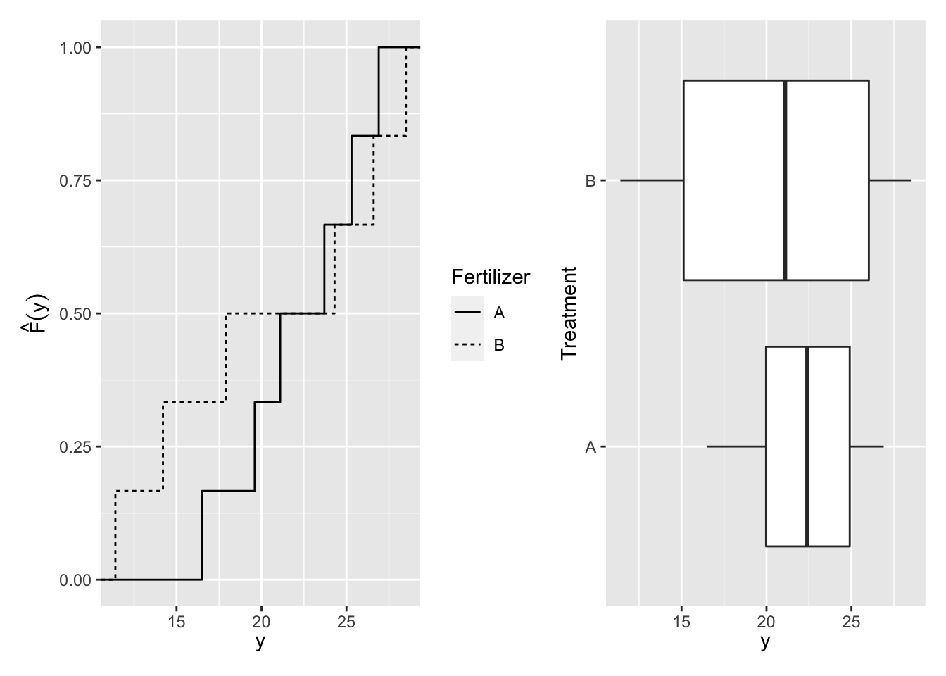
Figure 3.1: Distribution of Yield

Table 3.4: Random Shuffle of Treatment Assignment in Example 3.1

Plot 1, A, 11.4	Plot 4, B, 16.5	Plot 7, B, 26.9	Plot 10, B, 28.5
Plot 2, A, 23.7	Plot 5, A, 21.1	Plot 8, A, 26.6	Plot 11, A, 14.2
Plot 3, B, 17.9	Plot 6, B, 19.6	Plot 9, B, 25.3	Plot 12, A, 24.3

Is the difference in wheat yield due to the fertilizers or chance?

• Assume that there is no difference in the average yield between fertilizer A and fertilizer B.

• If there is no difference then the yield would be the same even if a different treatment allocation occurred.

• Under this assumption of no difference between the treatments, if one of the other 924 treatment allocations (e.g., A, A, B, B, A, B, B, A, B, B, A, A) was used then the treatments assigned to plots would have been randomly shuffled, but the yield in each plot would be exactly the same as in Table 3.2. This shuffled treatment allocation is shown in Table 3.4, and the difference in mean yield for this allocation is \(\delta=\) -2.23 (recall that the observed treatment difference \(\hat \delta^{obs} =\) 1.7).

A probability distribution for \(\delta = \bar y_A - \bar y_B\), called the randomization distribution, is constructed by calculating \(\delta\) for each possible randomization (i.e., treatment allocation).

Investigators are interested in determining whether fertilizer A produces a higher yield compared to fertilizer B, which corresponds to null and alternative hypotheses

\[\begin{aligned} & H_0: \text {Fertilizers A and B have the same mean wheat yield,} \\ & H_1: \text {Fertilizer B has a greater mean wheat yield than fertilizer A.} \end{aligned}\]

3.4.1 Computation Lab: Randomization Distribution

The data from Example 3.1 is in the fertdat data frame. The code chunk below computes the randomization distribution.

# 1. Number of possible randomizations

N <- choose(12,6) 

delta <- numeric(N) # Store the results

# 2. Generate N treatment assignments

trt_assignments <- combn(1:12,6) 

for (i in 1:N){
  # 3. compute mean difference and store the result
  
  delta[i] <- mean(fertdat$fert[trt_assignments[,i]]) - 
    mean(fertdat$fert[-trt_assignments[,i]])
}

1. N is the total number of possible treatment assignments or randomizations.

2. trt_assignments <- combn(1:12,6) generates all combinations of 6 elements taken from 1:12 (i.e., 1 through 12) as a \(6 \times 924\) matrix, where the \(i^{th}\) column trt_assignments[,i], \(i=1,\ldots,924\), represents the experimental units assigned to treatment A.

3. fertdat$fert[trt_assignments[,i]] selects fertdat$fert values indexed by trt_assignments[,i]. These values are assigned to treatment A. fertdat$fert[-trt_assignments[,i]] drops fertdat$fert values indexed by trt_assignments[,i]. These values are assigned to treatment B.

3.5 The Randomization p-value

3.5.1 One-sided p-value

Let \(T\) be a test statistic such as the difference between treatment means or medians. The p-value of the randomization test \(H_0: T=0\) can be calculated as the probability of obtaining a test statistic as extreme or more extreme than the observed value of the test statistic \(t^{*}\) (i.e., in favour of \(H_1\)). The p-value is the proportion of randomizations as extreme or more extreme than the observed value of the test statistic \(t^{*}\).

Definition 3.1 (One-sided Randomization p-value) Let \(T\) be a test statistic and \(t^{*}\) the observed value of \(T\). The one-sided p-value to test \(H_0:T=0\) is defined as:

\[\begin{aligned} P(T \ge t^{*})&= \sum_{i = 1}^{N \choose N_A} \frac{I(t_i \ge t^{*})}{{N \choose N_A}} \mbox{, if } H_1:T>0; \\ P(T \le t^{*})&=\sum_{i = 1}^{N \choose N_A} \frac{I(t_i \le t^{*})}{{N \choose N_A}} \mbox{, if } H_1:T<0. \end{aligned}\]

A hypothesis test to answer the question posed in Example 3.1 is \(H_0:\delta=0 \text{ v.s. } H_1:\delta>0,\) \(\delta=\bar y_A-\bar y_B.\) The observed value of the test statistic is 1.7.

3.5.2 Two-sided Randomization p-value

If we are using a two-sided alternative, then how do we calculate the randomization p-value? The randomization distribution may not be symmetric, so there is no justification for simply doubling the probability in one tail.

Definition 3.2 (Two-sided Randomization p-value) Let \(T\) be a test statistic and \(t^{*}\) the observed value of \(T\). The two-sided p-value to test \(H_0:T=0 \mbox{ vs. } H_1:T \ne 0\) is defined as:

\[P(\left|T\right| \ge \left|t^{*}|\right) = \sum_{i = 1}^{N \choose N_A} \frac{I(\left|t_i\right| \ge \left|t^{*}\right|)}{{N \choose N_A}}.\]

The numerator counts the number of randomizations where either \(t_i\) or \(-t_i\) exceed \(|t^{*}|\).

3.5.3 Computation Lab: Randomization p-value

The randomization distribution was computed in Section 3.4.1, and stored in delta. We want to compute the proportion of randomizations that exceed obs_diff.

glimpse(delta)
#>  num [1:924] -5.93 -3.5 -3.6 -4.03 -2.97 ...

delta >= obs_diff creates a Boolean vector that is TRUE if delta >= obs_diff, and FALSE otherwise, and sum applied to this Boolean vector counts the number of TRUE.

obs_diff
#> [1] 1.7
N
#> [1] 924
pval <- sum(delta >= obs_diff)/N
pval
#> [1] 0.303

The p-value can be interpreted as the proportion of randomizations that would produce an observed mean difference between A and B of at least 1.7 assuming the null hypothesis is true. In other words, under the assumption that there is no difference between the treatment means, 30.3% of randomizations would produce as extreme or more extreme difference than the observed mean difference of 1.7.

The two-sided p-value to test if there is a difference between fertilizers A and B in Example 3.1 can be computed as

pval2side <- sum(delta >= abs(obs_diff) | 
                   (-1)*delta >= abs(obs_diff))/N
pval2side
#> [1] 0.6061

In this case, the randomization distribution is roughly symmetric, so the two-sided p-value is approximately double the one-sided p-value.

The R code to produce Figure 3.2, without annotations, is shown below. The plot displays the randomization distribution of \(\delta=\bar y_A - \bar y_B\) for Example 3.1. The left panel shows the distribution using \(1-\hat F_{\delta}\), and the dotted line indicates how to read the p-value from this graph, and the right panel shows a histogram where the black bars show the values more extreme than the observed value.

p1 <- tibble(delta) %>%
  ggplot(aes(delta)) +
  geom_histogram(bins = 30, colour = "white", 
                 aes(y = ..count.. / sum(..count..))) +
  scale_x_continuous(breaks = seq(-10, 10, by = 2))

p2 <- tibble(delta) %>%
  ggplot(aes(delta)) + 
  geom_step(aes(y = 1 - ..y..), stat = "ecdf") +
  scale_y_continuous(breaks = seq(0, 1, by = 0.1)) +
  scale_x_continuous(breaks = seq(-10, 10, by = 2))

p2 + p1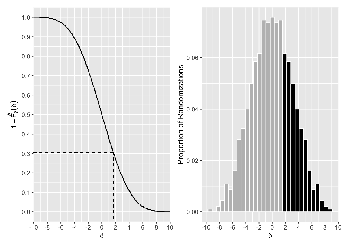

Figure 3.2: Randomization Distribution of Difference of Means

3.5.4 Randomization Confidence Intervals

Consider a completely randomized design comparing two groups where the treatment effect is additive. In Example 3.1, suppose that the yields for fertilizer A were shifted by \(\Delta\), these shifted responses; \(y_{i_A}-\Delta\) should be similar to \(y_{i_B}\) for \(i=1,\ldots,6,\) and the randomization test on these two sets of responses should not reject \(H_0\). In other words the difference between the distribution of yield for fertilizers A and B can be removed by subtracting \(\Delta\) from each plot assigned to fertilizer A.

Loosely speaking, a confidence interval, for the mean difference, consists of all the plausible values of the parameter \(\Delta\). A randomization confidence interval can be constructed by considering all values of \(\Delta_0\) for which the randomization test does not reject \(H_0:\Delta=\Delta_0 \mbox{ vs. } H_a:\Delta \ne\Delta_0\).

Definition 3.3 (Randomization Confidence Interval) Let \(T_{\Delta}\) be the test statistic calculated using the treatment responses for treatment A shifted by \(\Delta\), \(t^{*}\) its observed value, and \(p(\Delta)=F_{T_{\Delta}}(t^{*}_{\Delta})=P(T_{\Delta}\leq t^{*}_{\Delta})\) be the observed value of the CDF as a function of \(\Delta\).

A \(100(1-\alpha)\%\) randomization confidence interval for \(\Delta\) can then be obtained by inverting \(p(\Delta)\). A two-sided \(100(1-\alpha)\%\) is \((\Delta_L,\Delta_U)\), where \(\Delta_L=p^{-1}(\alpha/2)=\max_{p(\Delta \leq \alpha/2)} \Delta\), and \(\Delta_U=p^{-1}(1-\alpha/2)=\min_{p(\Delta \leq 1-\alpha/2)} \Delta\).²⁹

3.5.5 Computation Lab: Randomization Confidence Intervals

Computing \(\Delta_L, \Delta_U\) involves recomputing the randomization distribution of \(T_{\Delta}\) for a series of values \(\Delta_1,\ldots,\Delta_k\). This can be done by trial and error, or by a search method (see for example Paul H Garthwaite³⁰).

In this section, a trial and error method is implemented using a series of R functions.

The function randomization_dist() computes the randomization distribution for the mean difference in a randomized two-sample design.

randomization_dist <- function(dat, M, m) {
  N <- choose(M, m)
  randdist <- numeric(N)
  trt_assignments <- combn(1:M, m)
  for (i in 1:N) {
    randdist[i] <-
      mean(dat[trt_assignments[, i]]) - 
      mean(dat[-trt_assignments[, i]])
  }
  return(randdist)
}

The function randomization_pctiles() computes \(p(\Delta)\) for a sequence of trial values for \(\Delta\).

randomization_pctiles <- function(delta, datA, datB, M, m) {
  pctiles <- numeric(length(delta))
  for (i in 1:length(delta)) {
    yA <- datA + delta[i]
    yB <- datB
    obs_diff <- mean(yA) - mean(yB)
    dat <- c(yA, yB)
    y <- randomization_dist(dat, M, m)
    pctiles[i] <- sum(y <= obs_diff) / N
  }
  return(pctiles)
}

The function randomization_ci() computes the \(\Delta_L,\Delta_U\) as well as the confidence level of the interval.

randomization_ci <- function(alpha, delta, yB, yA, M, m) {
  ptiles <- randomization_pctiles(delta, yB, yA, M, m)
  L <- sum(ptiles <= alpha / 2)
  U <- sum(ptiles <= (1 - (alpha / 2)))
  Lptile <- ptiles[L]
  Uptile <- ptiles[U]
  LCI <- delta[L]
  UCI <- delta[U]
  conf_level <- Lptile + 1 - Uptile
  return(data.frame(Lptile, Uptile, conf_level, LCI, UCI))
}

Example 3.2 (Confidence interval for wheat yield in Example 3.1) A 99% randomization confidence interval for the wheat data can be obtained by using randomization_ci(). The data for the two groups are defined by yA and yB, the confidence level is alpha, with M total experimental units and m experimental units in one of the groups. The sequence of values for \(\Delta\) is found by trial and error, but it’s important that the tails of the distribution of \(\Delta\) are computed far enough so that we have values for the upper and lower \(\alpha/2\) percentiles.

A plot of \(p(\Delta)\) is shown in Figure 3.3. delta is selected so that pdelta is computed in tails of the distribution of \(T_{\Delta}.\)

alpha <- 0.01
delta <- seq(-16,16,by=0.1)
M <- 12
m <- 6
yA <- fertdat$fert[fertdat$shuffle=="A"]
yB <- fertdat$fert[fertdat$shuffle=="B"]

tibble(pdelta = randomization_pctiles(delta = delta, 
                                      datA = yA, 
                                      datB = yB, 
                                      M = M, 
                                      m = m)) %>%
  ggplot(aes(delta, pdelta)) + geom_point()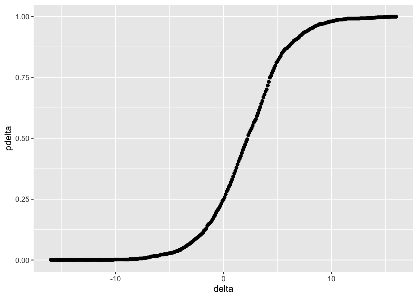

Figure 3.3: Distribution of \(\Delta\) in Example 3.2

randomization_ci(alpha, delta, yA,yB, M, m)
#>     Lptile Uptile conf_level LCI UCI
#> 1 0.004329 0.9946    0.00974  -8  14

Lptile and Uptile are the lower and upper percentiles of the distribution of \(T_{\Delta}\) used for the confidence interval, conf_level is actual confidence level of the confidence interval, and finally LCI, UCI are the limits of a (\(1-\)conf_level) level confidence interval. In this case, \((\Delta_L, \Delta_U)=(-8, 14)\) is a 99.03% confidence interval for the difference between the means of treatments A and B.

3.6 Randomization Distribution of a Test Statistic

Test statistics other than \(T={\bar y}_A-{\bar y}_B\) could be used to measure the effectiveness of fertilizer A in Example 3.1. Investigators may wish to compare differences between medians, standard deviations, odds ratios, or other test statistics.

3.6.1 Computation Lab: Randomization Distribution of a Test Statistic

The randomization distribution of the difference in group medians can be obtained by modifying the randomization_dist() function (see 3.5.5) used to calculate the difference in group means. We can add func as an argument to randomization_dist() and modify the function so that the type of difference can be specified.

randomization_dist <- function(func, dat, M, m) {
  N <- choose(M, m)
  randdist <- numeric(N)
  trt_assignments <- combn(1:M, m)
  for (i in 1:N) {
    randdist[i] <-
      (func(dat[trt_assignments[, i]]) -
         func(dat[-trt_assignments[, i]]))
  }
  return(randdist)
}

The randomization distribution of the difference in medians is

randdist_median <- randomization_dist(median, fertdat$fert, 12, 6)

The p-value of the randomization test comparing two medians is

obs_median_diff <- median(yA) - median(yB)
pval <- sum(randdist_median >= obs_median_diff)/N
pval
[1] 0.5195

3.7 Computing the Randomization Distribution using Monte Carlo Sampling

Computation of the randomization distribution involves calculating the test statistic for every possible way to split the data into two samples of size \(N_A\). If \(N = 100\) and \(N_A = 50\), this would result in \({100 \choose 50}=\) 1.0089^{20} billion differences. These types of calculations are not practical unless the sample size is small.

Instead, we can resort to Monte Carlo sampling from the randomization distribution to estimate the exact p-value.

The data set can be randomly divided into two groups and the test statistic calculated. Several thousand test statistics are usually sufficient to get an accurate estimate of the exact p-value and sampling can be done without replacement.

If \(M\) test statistics, \(t_i\), \(i = 1,...,M\) are randomly sampled from the permutation distribution, a one-sided Monte Carlo p-value for a test of \(H_0: \mu_T = 0\) versus \(H_1: \mu_T > 0\) is

\[ {\hat p} = \frac {1+\sum_{i = 1}^M I(t_i \ge t^{*})}{M+1}.\]

Including the observed value \(t^{*}\) there are \(M+1\) test statistics.

3.7.1 Computation Lab: Calculating the Randomization Distribution using Monte Carlo Sampling

Example 3.3 (What is the effect of caffeine on reaction time?) There is scientific evidence that caffeine reduces reaction time Tom M McLellan, John A Caldwell, and Harris R Lieberman³¹. A study of the effects of caffeine on reaction time was conducted on a group of 100 high school students. The investigators randomly assigned an equal number of students to two groups: one group (CAFF) consumed a caffeinated beverage prior to taking the test, and the other group (NOCAFF) consumed the same amount of water. The research objective was to study the effect of caffeine on reaction time to test the hypothesis that caffeine would reduce reaction time among high school students. The data from the study is in the data frame rtdat.

ggplot(rtdat, aes(rt, group)) + geom_boxplot()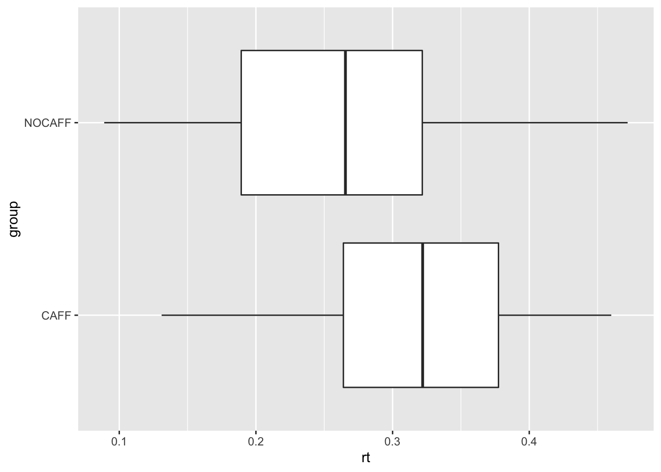

The data indicate that the difference in median reaction times between the CAFF and NOCAFF groups is 0.056 seconds. Is the observed difference due to random chance or is there evidence it is due to caffeine? Let’s try to calculate the randomization distribution using randomization_dist().

randomization_dist(func = mean, dat = rt, M = 100, m = 50)
Error in numeric(N): vector size specified is too large

Currently, R can only support vectors up to \(2^{52}\) elements,³² so computing the full randomization distribution becomes much more difficult. In this case, Monte Carlo sampling provides a feasible way to approximate the randomization distribution and p-value.

caff <- rtdat$rt[rtdat$group == "CAFF"]
ncaff <- rtdat$rt[rtdat$group == "NOCAFF"]
rt1 <- c(caff, ncaff)
N <- 10000
result <- numeric(N)

for (i in 1:N) {
  index <- sample(length(rt), 
                  size = length(caff), 
                  replace = FALSE)
  result[i] <- median(rt[index]) - median(rt[-index])
}

observed <- median(caff) - median(ncaff)
phatval <- (sum(result >= observed) + 1) / (N + 1)
phatval
#> [1] 0.0038

A p-value equal to 0.004 indicates that the median difference is unusual assuming the null hypothesis is true. Thus, this study provides evidence that caffeine slows down reaction time.

3.8 Properties of the Randomization Test

The p-value of the randomization test must be a multiple of \(1/{\binom{N} {N_A}}\). If a significance level of \(\alpha=k/{\binom{N} {N_A}}\), where \(k = 1,...,{N \choose N_A}\) is chosen, then \(P(\text{type I}) = \alpha.\) In other words, the randomization test is an exact test.

If \(\alpha\) is not chosen as a multiple of \(1/{\binom {N}{N_A}}\), but \(k/{\binom {N}{N_A}}\) is the largest p-value less than \(\alpha\), then \(P(\text{type I}) = k/{\binom {N}{N_A}}< \alpha\), and the randomization test is conservative. Either way, the test is guaranteed to control the probability of a type I error under very minimal conditions: randomization of the experimental units to the treatments.³³

3.9 The Two-sample t-test

Consider designing a study where the primary objective is to compare a continuous variable in each group. Let \(Y_{ik}\) be the observed outcome for the \(i^{th}\) experimental unit in the \(kth\) treatment group, for \(i = 1,...,n_k\) and \(k= 1,2\). The outcomes in the two groups are assumed to be independent and normally distributed with different means but an equal variance \(\sigma^2\), \(Y_{ik} \sim N(\mu_k,\sigma^2).\)

Let \(\theta=\mu_1-\mu_2\), be the difference in means between the two treatments. \(H_0:\theta =\theta_0 \mbox{ vs. }H_1:\theta \ne \theta_0\) specify a hypothesis test to evaluate whether the evidence shows that the two treatments are different.

The sample mean for each group is given by \({\bar Y}_k = (1/n_k)\sum_{i = 1}^{n_k} Y_{ik}\), \(k = 1,2\), and the pooled sample variance is

\[S^2_p= \frac{(n_1-1)S_1^2 + (n_2-1)S_2^2}{(n_1+n_2-2)},\] where \(S_k^2\) is the sample variance for group \(k=1,2.\)

The two-sample t statistic is given by

\[\begin{equation} T=\frac {{\bar Y}_1 - {\bar Y}_2 - \theta_0}{S_p \sqrt{(1/n_1+1/n_2)}} \tag{3.1}. \end{equation}\]

When \(H_0\) is true, \(T \sim t_{n_1+n_2-2}.\)

For example, the two-sided p-value for testing \(\theta\) is \(P\left(|t_{n_1+n_2-2}|>|T^{obs}|\right)\), where \(T^{obs}\) is the observed value of (3.1). The hypothesis testing procedure assesses the strength of evidence contained in the data against the null hypothesis. If the p-value is adequately small, say, less than 0.05 under a two-sided test, we reject the null hypothesis and claim that there is a significant difference between the two treatments; otherwise, there is no significant difference and the study is inconclusive.

In Example, 3.1 \(H_0:\mu_A=\mu_B\) and \(H_1: \mu_A < \mu_B.\) The pooled sample variance and the observed value of the two-sample t-statistic for this example are:

\[S_p^2 = \frac{(n_1-1)S_1^2+(n_2-1)S_2^2}{n_1+n_2-2} = 5.65,\] and \[T^{obs} = \frac {{\bar y}_A - {\bar y}_b}{S_p \sqrt{(1/n_A+1/n_B)}} = \frac {20.22 - 22.45}{5.65 \sqrt{(1/6+1/6)}}=-0.69.\]

The p-value is \(P\left(t_{10} < -0.69\right)=\) 0.3. There is little evidence that fertilizer A produces higher yields than B.

3.9.1 Computation Lab: Two-sample t-test

We can use R to compute the p-value of the two-sample t-test for Example 3.1. Recall that the data frame fertdat contains the data for this example: fert is the yield and shuffle is the treatment.

glimpse(fertdat)
#> Rows: 12
#> Columns: 2
#> $ fert    <dbl> 11.4, 23.7, 17.9, 16.5, 21.1, 19.6, 2…
#> $ shuffle <chr> "A", "A", "B", "B", "A", "B", "B", "A…

The pooled variance \(s_p^2\) and observed value of the two-sample t statistic are:

yA <- fertdat$fert[fertdat$shuffle == "A"]
yB <- fertdat$fert[fertdat$shuffle == "B"]

n1 <- length(yA) - 1
n2 <- length(yB) - 1

sp <- sqrt(((n1 - 1)*var(yA) + (n2 - 1)*var(yB))/(n1 + n2 -2))

sp
#> [1] 5.595

tobs <- (mean(yA)-mean(yB))/(sp*sqrt(1/6 + 1/6))
tobs
#> [1] -0.6914

The observed value of the two-sample t-statistic is -0.6914.

Finally, the p-value for this test can be calculated using the CDF of the \(t_n\), where \(n = 6 + 6 -2=10.\)

df <- 6 + 6 - 2
pt(tobs, df)
#> [1] 0.2525

These calculations are also implemented in stats::t.test().

t.test(yA, yB, var.equal = TRUE, alternative = "less")
#> 
#>  Two Sample t-test
#> 
#> data:  yA and yB
#> t = -0.69, df = 10, p-value = 0.3
#> alternative hypothesis: true difference in means is less than 0
#> 95 percent confidence interval:
#>   -Inf 3.621
#> sample estimates:
#> mean of x mean of y 
#>     20.22     22.45

The assumption of normality can be checked using normal quantile plots, although the t-test is robust against non-normality.

fertdat %>%
  ggplot(aes(sample = fert, linetype = shuffle)) +
  geom_qq(aes(shape = shuffle)) +
  geom_qq_line() +
  ggtitle("Normal Quantile Plot")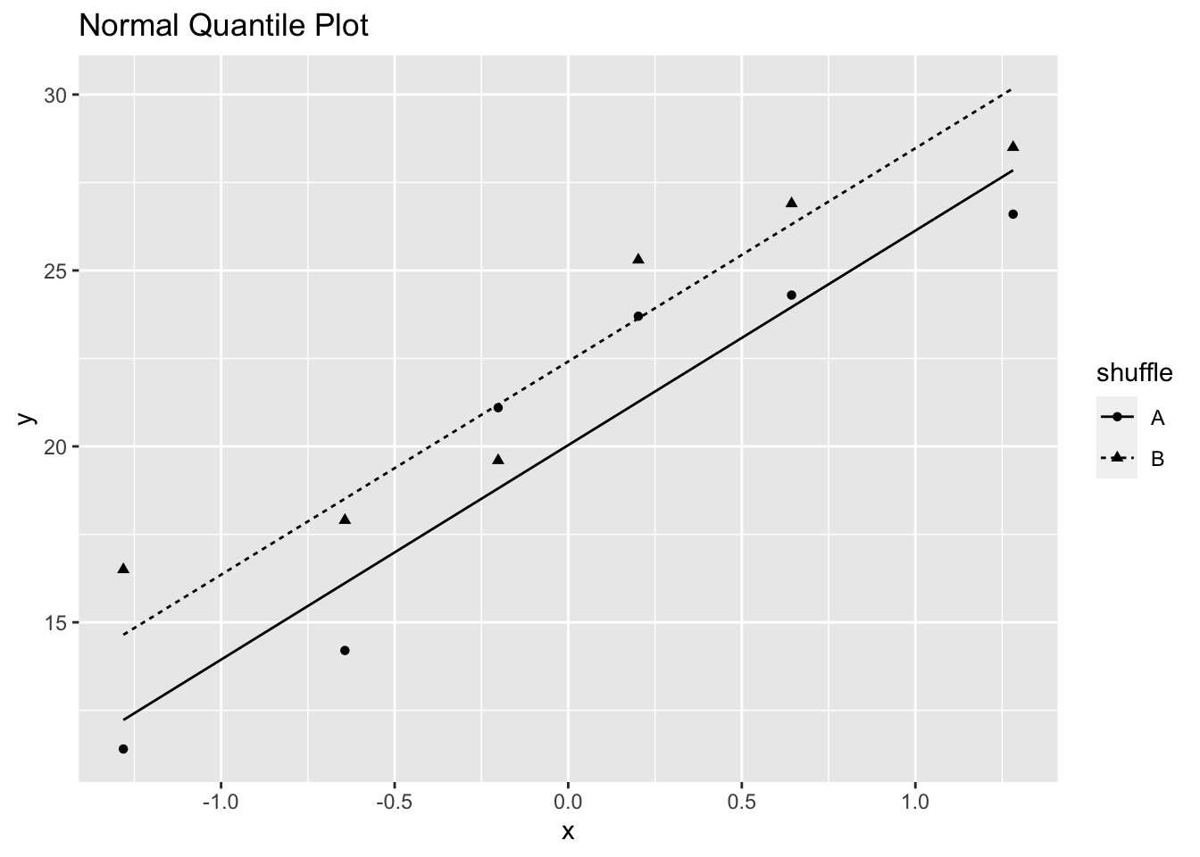

Figure 3.4: Normal Quantile Plot of Fertilizer Yield in Example 3.1

Figure 3.4 indicates that the normality assumption is satisfied, although the sample sizes are fairly small.

Notice that the p-value from the randomization test and the p-value from two-sample t-test are almost identical although the randomization test neither depends on normality nor independence. The randomization test does depend on Fisher’s concept that after randomization, if the null hypothesis is true, the two results obtained from each particular plot will be exchangeable. The randomization test tells you what you could say if exchangeability were true.

3.10 Blocking

Randomizing subjects to two treatments should produce two treatment groups where all the covariates are balanced (i.e., have similar distributions), but it doesn’t guarantee that the treatment groups will be balanced on all covariates. In many applications there may be covariates that are known a priori to have an effect on the outcome, and it’s important that these covariates be measured and balanced, so that the treatment comparison is not affected by the imbalance in these covariates. Suppose an important covariate is income level (low/medium/high). If income level is related to the outcome of interest, then it’s important that the two treatment groups have a balanced number of subjects in each income level, and this shouldn’t be left to chance. To avoid an imbalance between income levels in the two treatment groups, the design can be blocked by income group, by separately randomizing subjects in low, medium, and high income groups.

Example 3.4 Young-Woo Kim et al.³⁴ conducted a randomized clinical trial to evaluate hemoglobin level (an important component of blood) levels after a surgery to remove a cancer. Patients were randomized to receieve a new treatment or placebo. The study was conducted at seven major institutions in the Republic of Korea. Previous research has shown that the amount of cancer in a person’s body, measured by cancer stage (stage I—less cancer, stages II—IV - more cancer), has an effect on hemoglobin. 450 (225 per group) patients were required to detect a significant difference in the main study outcome at the 5% level (with 90% power - see Chapter—4).

To illustrate the importance of blocking, consider a realistic, although hypothetical, scenario related to Example 3.4. Suppose that among patients eligible for inclusion in the study, 1/3 have stage I cancer, and 225 (50%) patients are randomized to the treatment and placebo groups. Table 3.5 shows that the distribution of Stage in the placebo group is different than the distribution in the Treatment group. In other words, the distribution of cancer stage in each treatment group is unbalanced. The imbalance in cancer stage might create a bias when comparing the two treatment groups since it’s known a priori that cancer stage has an effect on the main study outcome (hemoglobin level after surgery). An unbiased comparison of the treatment groups would have Stage balanced between the two groups.

Table 3.5: Distribution of Cancer Stage by Treatment Group in Example 3.4 using Unrestricted Randomization

Stage	Placebo	Treatment
Stage I	70	80
Stage II-IV	155	145

How can an investigator guarantee that Stage is balanced in the two groups? Separate randomizations by cancer stage, blocking by cancer stage.

3.11 Treatment Assignment in Randomized Block Designs

If Stage was balanced in the two treatment groups in Example 3.4, then 50% of stage I patients would receive Placebo, and 50% Treatment. If we block or separate the randomizations by Stage, then this will yield treatment groups balanced by stage. There will be \(150 \choose 75\) randomizations for the stage I patients, and \(300 \choose 150\) randomizations for the stage II-IV patients. Table 3.6 shows the results of block randomization.

Table 3.6: Distribution of Cancer Stage by Treatment Group in Example 3.4 using Restricted Randomization

Stage	Placebo	Treatment
Stage I	75	75
Stage II-IV	150	150

3.11.1 Computation Lab: Generating a Randomized Block Design

Let’s return to Example 3.4, and suppose that we are designing a study where 450 subjects will be randomized to two treatments, and 1/3 of the 450 subjects (150) have stage I cancer. cancerdat is a data frame containing a patient id and Stage information.

cancerdat_stageI <- data.frame(id = 1:150)

First, we will create a data frame, cancerdat_stageI of patient id with stage I cancers. Next, randomly select 50% of patient id in this block sample(cancerdat_stageI$id, floor(nrow(cancerdat_stageI)/2)) and assign these patients to Treatment, and the remaining to Placebo using treat = ifelse(id %in% trtids, "Treatment", "Placebo").

trtids <-
  sample(cancerdat_stageI$id, floor(nrow(cancerdat_stageI) / 2))

cancerdat_Ibl <-
  mutate(cancerdat_stageI,
         treat = ifelse(id %in% trtids, "Treatment", "Placebo"))

The treatment assignments for the first 4 patients with stage I cancer are shown below.

cancerdat_Ibl %>% head(n = 4)
#>   id   Stage     treat
#> 1  1 Stage I   Placebo
#> 2  2 Stage I   Placebo
#> 3  3 Stage I Treatment
#> 4  4 Stage I Treatment

3.12 Randomized Matched Pairs Design

A randomized matched pairs design arranges experimental units in pairs, and treatment is randomized within a pair. In other words, each experimental unit is a block. In Chapter 5, we will see how this idea can be extended to compare more than two treatments using randomized block designs.

Example 3.5 (Wear of boys' shoes) Measurements on the amount of wear of the soles of shoes worn by 10 boys were obtained by the following design (this example is based on 3.2 in George EP Box, J Stuart Hunter, and William Gordon Hunter³⁵).

Each boy wore a special pair of shoes with the soles made of two different synthetic materials, A (a standard material) and B (a cheaper material). The left or right sole was randomly assigned to A or B, and the amount of wear after one week was recorded (a smaller value means less wear). During the test some boys scuffed their shoes more than others, but each boy’s shoes were subjected to the same amount of wear.

In this case, each boy is a block, and the two treatments are randomized within a block.

Material was randomized to the left or right shoe by flipping a coin. The observed treatment assignment is one of \(2^{10}=1,024\) equiprobable treatment assignments.

The observed mean difference is 1.7. Figure 3.5, a connected dot plot of wear for each boy, shows material B had higher wear for most boys.

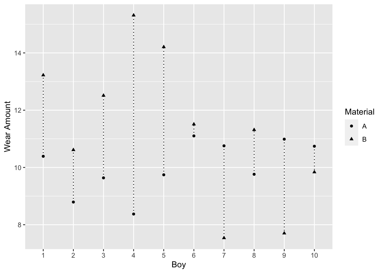
Figure 3.5: Boy’s Shoe Example

3.13 Randomized Matched Pairs versus Completely Randomized Design

Ultimately, the goal is to compare units that are similar except for the treatment they were assigned. So, if groups of similar units can be created before randomizing, then it’s reasonable to expect that there should be less variability between the treatment groups. Blocking factors are used when the investigator has knowledge of a factor before the study that is measurable and might be strongly associated with the dependent variable.

The most basic blocked design is the randomized pairs design. This design has \(n\) units where two treatments are randomly assigned to each unit which results in a pair of observations \((X_i,Y_i), i=1,\ldots,n\) on each unit. In this case, each unit is a block. Assume that the \(X's\) and \(Y's\) have means \(\mu_X\) and \(\mu_Y\), and variances \(\sigma^2_X\) and \(\sigma^2_Y\), and the pairs are independently distributed and \(Cov(X_i,Y_i)=\sigma_{XY}\). An estimate of \(\mu_X-\mu_Y\) is \(\bar D = \bar X - \bar Y\). It follows that

\[\begin{align} \begin{split} E\left(\bar D \right) &= \mu_X-\mu_Y \\ Var\left(\bar D \right) &= \frac{1}{n}\left(\sigma^2_X + \sigma^2_Y - 2\rho\sigma_X\sigma_Y \right), \end{split} \tag{3.2} \end{align}\]

where \(\rho\) is the correlation between \(X\) and \(Y\).

Alternatively, if \(n\) units had been assigned to two independent treatment groups (i.e., \(2n\) units) then \(Var\left(\bar D\right)=(1/n) \left(\sigma^2_X+\sigma^2_Y\right).\) Comparing the variances we see that the variance of \(\bar D\) is smaller in the paired design if the correlation is positive. So, pairing is a more effective experimental design.

3.14 The Randomization Test for a Randomized Paires Design

Table 3.7: Possible Randomizations for Example 3.5

Observed	L	L	R	R	R	L	R	R	L	L
Possible	R	R	R	R	L	R	R	R	L	L
Wear (A)	10.39	8.79	9.64	8.37	9.74	11.1	10.76	9.76	10.99	10.74
Wear (B)	13.22	10.61	12.51	15.31	14.21	11.51	7.54	11.31	7.7	9.84

Table 3.7 shows the observed (randomization) and another possible (randomization) for material A in Example 3.5. If the other possible randomization was observed, then \(\bar y_A - \bar y_B =\) -1.4.

The differences \(\bar y_A - \bar y_B\) can be analyzed so that we have one response per boy. Under the null hypothesis, the wear of a boy’s left or right shoe is the same regardless of what material he had on his sole, and the material assigned is based on the result of, for example, a sequence of ten tosses of a fair coin (e.g., in R this could be implemented by sample(x = c("L","R"),size = 10,replace = TRUE)). This means that under the null hypothesis if the Possible Randomization in Table 3.7 was observed, then for the first boy the right side would have been assigned material A and the left side material B, but the amount of wear on the left and right shoes would be the same, so the difference for the first boy would have been 2.8 instead of -2.8 since his wear for materials A and B would have been 13.22 and 10.39 respectively.

The randomization distribution is obtained by calculating 1,024 averages \(\bar y_A-\bar y_B = (\pm\) -2.8 \(\pm\) -1.8 \(\pm \cdots \pm\) 0.9 \()/\) 10, corresponding to each of the \(2^{10}=1,024\) possible treatment assignments.

3.14.1 Computation Lab: Randomization Test for a Paired Design

The data for Example 3.5 is in shoedat_obs data frame.

head(shoedat_obs , n = 3)
#>   boy sideA sideB  wearA wearB
#> 1   1     L     R 10.390 13.22
#> 2   2     L     R  8.792 10.61
#> 3   3     R     L  9.636 12.51

The code chunk below generates the randomization distribution.

diff <- shoedat_obs %>%
  mutate(diff = wearA - wearB) %>%
  select(diff) %>%
  unlist() # calculate difference

N <- 2 ^ (10) # number of treatment assignments

res <- numeric(N) #vector to store results

LR <- list(c(-1, 1)) # difference is multiplied by -1 or 1

# generate all possible treatment assign
trtassign <- expand.grid(rep(LR, 10))

for (i in 1:N) {
  res[i] <- mean(as.numeric(trtassign[i, ]) * diff)
}

The \(2^{10}\) treatment assignments are computed using expand.grid() on a list of 10 vectors (c(-1,1))—each element of the list is the potential sign of the difference for one experimental unit (i.e., boy), and expand.grid() creates a data frame from all combinations of these 10 vectors.

tibble(res) %>% 
  ggplot(aes(res)) + 
  geom_histogram(bins=20, colour = "black", fill = "grey") +
  xlab("Mean Difference") + 
  geom_vline(aes(xintercept = obs_diff), size =1.5)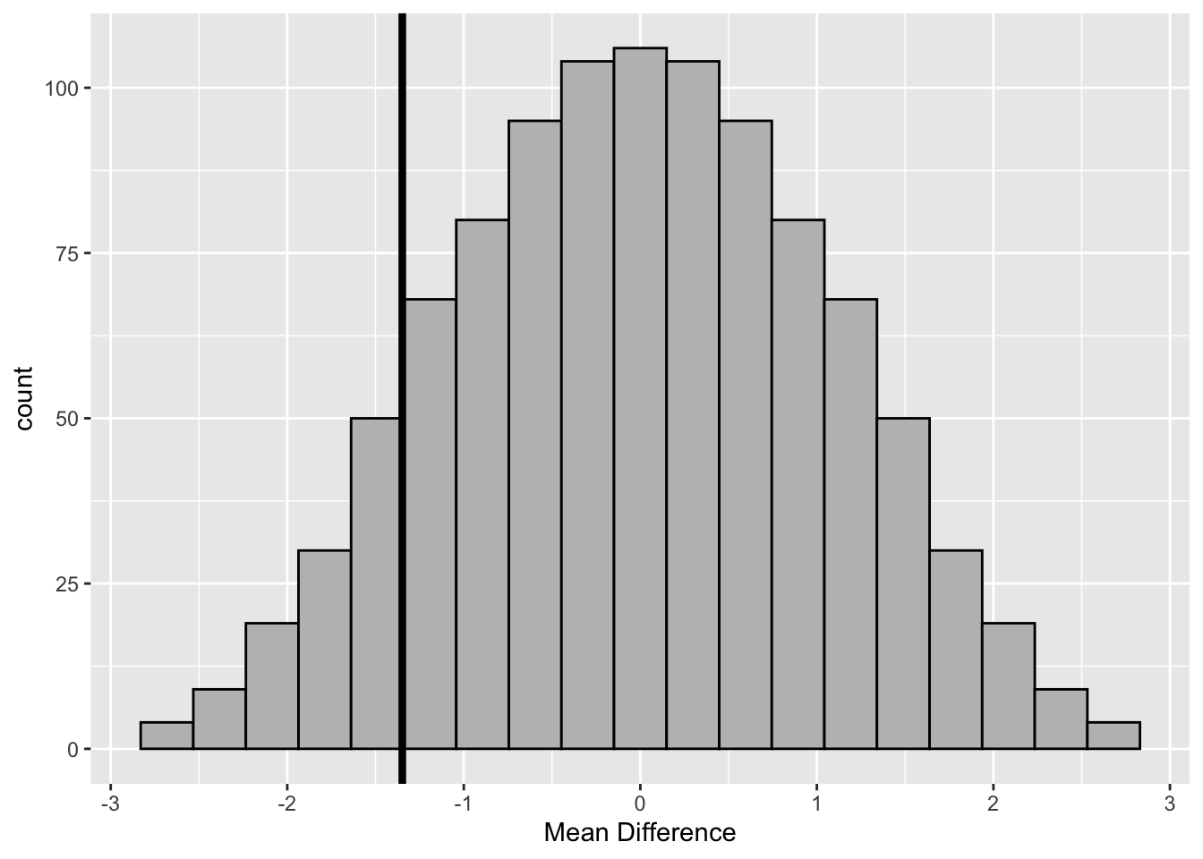

Figure 3.6: Randomization Distribution–Boys’ Shoes

The p-value for testing if B has more wear than A is

\[P(D \le d^{*})= \sum_{i = 1}^{2^{10}} \frac{I(d_i \le d^{*})}{2^{10}},\]

where \(D={\bar y_A}-{\bar y_B}\), and \(d^{*}\) is the observed mean difference.

sum(res <= obs_diff) / N # p-value
#> [1] 0.1084

The value of \(d^{*}=\) -1.3 is not unusual under the null hypothesis since only 111 (i.e., 10%) differences of the randomization distribution are less than -1.3. Therefore, there is no evidence of a significant increase in the amount of wear with the cheaper material B.

3.15 Paired t-test

If we assume that the differences from Example 3.5 are a random sample from a normal distribution, then \(t=\sqrt{10}{\bar d}/S_{\bar d} \sim t_{10-1},\) where, \(S_{\bar d}\) is the sample standard deviation of the paired differences. The p-value for testing if \({\bar D} < 0\) is \(P(t_{9}< t).\) In other words, this is the same as a one-sample t-test of the differences.

3.15.1 Computation Lab: Paired t-test

In Section 3.14.1, diff is a vector of the differences for each boy in Example 3.5. The observed value of the t-statistic for the one-sample test can be computed.

n <- length(diff)
t_pair_obs <- sqrt(n) * mean(diff) / sd(diff)
t_pair_obs
#> [1] -1.319

The p-value for testing \(H_0:{\bar D} = 0\) versus \(H_a:{\bar D} < 0\) is

df <- n - 1
pt(t_pair_obs, df)
#> [1] 0.1099

Alternatively, t.test() can be used.

t.test(diff, alternative = "less") 
#> 
#>  One Sample t-test
#> 
#> data:  diff
#> t = -1.3, df = 9, p-value = 0.1
#> alternative hypothesis: true mean is less than 0
#> 95 percent confidence interval:
#>    -Inf 0.5257
#> sample estimates:
#> mean of x 
#>    -1.348

3.16 Exercises

Exercise 3.1 Suppose \(X_1\sim N\left(10, 25\right)\) and \(X_2\sim N\left(5, 4\right)\) in a population. You randomly select 100 samples from the population and assign treatment A to half of the sample and B to the rest. Simulate the sample with treatment assignments and the covariates, \(X_1\) and \(X_2\). Compare the distributions of \(X_1\) and \(X_2\) in the two treatment groups. Repeat the simulation one hundred times. Do you observe consistent results?

Exercise 3.2 Identify treatments and experimental units in the following scenarios.

1. City A would like to evaluate whether a new employment training program for the unemployed is more effective compared to the existing program. The City decides to run a pilot program for selected employment program applicants.

2. Marketing Agency B creates and places targeted advertisements on video-sharing platforms for its clients. The Agency decides to run an experiment to compare the effectiveness of placing advertisements before vs. during vs. after videos.

3. Paul enjoys baking and finds a new recipe for chocolate chip cookies. Paul decides to test it by bringing cookies baked using his current recipe and the new recipe to his study group. Each member of the group blindly tastes each kind and provides their ratings.

Exercise 3.3 A study has three experimental units and two treatments—A and B. List all possible treatment assignments for the study. How many are there? In general, show that there are \(2^N\) possible treatment assignments for an experiement with \(N\) experimenal units and 2 treatments.

Exercise 3.4 Consider the scenario in Example 3.1, and suppose that an investigator only has enough fertilizer A to use on four plots. Answer the following questions.

1. What is the probability that an individual plot receives fertilizer A?

2. What is the probability of choosing the treatment assignment A, A, A, A, B, B, B, B, B, B, B, B?

Exercise 3.5 Show that the one-sided p-value is \(1-\hat{F}_T\left(t^*\right)\) if \(H_1:T>0\) and \(\hat{F}_T\left(t^*\right)\) if \(H_1:T<0\), where \(\hat{F}_T\) is the ECDF of the randomization distribution of \(T\) and \(t^*\) is the observed value of \(T\).

Exercise 3.6 Show that the two-sided p-value is \(1-\hat{F}_T\left(\lvert t^*\rvert\right)+\hat{F}_T\left(-\lvert t^*\rvert\right)\), where \(\hat{F}_T\) is the ECDF of the randomization distribution of \(T\) and \(t^*\) is the observed value of \(T\).

Exercise 3.7 The actual confidence level conf_level does not equal the theoretical confidence level 0.01 in Example 3.2. Explain why.

Exercise 3.8 Consider Example 3.5. For each of the 10 boys, we randomly assigned the left or right sole to material A and the remaining side to B. Use R’s sample function to simulate a treatment assignment.

Exercise 3.9 Recall that the randomization test for the data in Example 3.5 fails to find evidence of a significant increase in the amount of wear with material B. Does this mean that material B has equivalent wear to material A? Explain.

Exercise 3.10 Consider the study from Example 3.4. Recall that the clinical trial consists of 450 patients. 150 of the patients have stage I cancer and the rest have stages II-IV cancer. In Computation Lab: Generating a Randomized Block Design, we created a balanced treatment assignment for the stage I cancer patients.

1. Create a balanced treatment assignment for the stage II-IV cancer patients.

2. Combine treatment assignments for stage I and stage II-IV. Show that the distribution of stage is balanced in the overall treatment assignment.

Exercise 3.11 Consider a randomized pair design with \(n\) units where two treatments are randomly assigned to each unit, resulting in a pair of observations \(\left(X_i,Y_i\right)\), for \(i=1,\ldots,n\) on each unit. Assume that \(E[X_i]=\mu_X\), \(E[Y_i]=\mu_y\), and \(Var(X_i)=Var(Y_i)=\sigma^2\) for \(i=1,\dots,n\). Alternatively, we may consider an unpaired design where we assign two independent treatment groups to \(2n\) units.

1. Show that the ratio of the variances in the paired to the unpaired design is \(1-\rho\), where \(\rho\) is the correlation between \(X_i\) and \(Y_i\).

2. If \(\rho=0.5\), how many subjects are required in the unpaired design to yield the same precision as the paired design?

Exercise 3.12 Suppose that two drugs A and B are to be tested on 12 subjects’ eyes. The drugs will be randomly assigned to the left eye or right eye based on the flip of a fair coin. If the coin toss is heads then a subject will receive drug A in their right eye. The coin was flipped 12 times and the following sequence of heads and tails was obtained:

\[\begin{array} {c c c c c c c c c c c c} T&T&H&T&H&T&T&T&H&T&T&H \end{array}\]

1. Create a table that shows how the treatments will be allocated to the 12 subjects’ left and right eyes.

2. What is the probability of obtaining this treatment allocation?

3. What type of experimental design has been used to assign treatments to subjects? Explain.

#> 
#> Attaching package: 'dplyr'
#> The following objects are masked from 'package:stats':
#> 
#>     filter, lag
#> The following objects are masked from 'package:base':
#> 
#>     intersect, setdiff, setequal, union