4 Power and Sample Size

4.1 Introduction

Consider a scenario where a continuous study outcome, with variance equal to one, is measured in two groups. The group means are \(\mu_1\) and \(\mu_2\). An investigator tests \(H_0:\mu_1-\mu_2=0\) versus \(H_1:\mu_1 \ne\mu_2\) with a sample of fifteen experimental units in each group.

The function my_ttest() simulates data to test this hypothesis with a t-test, where \(\mu_1=0\), \(\mu_2=0.1\), and \(\sigma^2=1\) in both groups.

my_ttest <- function(sampsize) {
  set.seed(6)
  x1 <- rnorm(sampsize, mean = 0, sd = 1)
  x2 <- rnorm(sampsize, mean = 0.1, sd = 1)
  myttest <- t.test(x1, x2, var.equal = TRUE)
  return(myttest$p.value) 
  }

The simulation below shows that the t-test failed to detect a significant difference even though a difference exists (i.e., \(H_0\) is false).

my_ttest(15)
#> [1] 0.4446615

In this case, we know \(\mu_1 \ne \mu_2\), so why does the the p-value indicate that there is no difference between the group means? Let’s change the sample size to 1,000 per group.

my_ttest(1000)
#> [1] 0.004706338

Now, the p-value indicates that there is strong evidence that \(H_0\) is false. The test failed to detect a difference when the sample size was 15 due to low power, and in this case, low power is due to a small sample size in each group.

Power is important in many fields of study. Suppose that researchers would like to compare two versions of a web page to investigate whether one page leads to an increase in sales. A pharmaceutical company is comparing a novel treatment for cancer against the standard treatment to investigate whether patient mortality decreases when receiving the novel treatment. A psychologist is studying how physical expression influences psychological processes such as risk taking, so she plans to randomize subjects into two groups where one group was instructed to pose in a high-power (this has nothing to do with statistical power) position and the second group in a low-power position. In all these scenarios, the investigators can calculate how many experimental units are required so that the statistical test used will have a high probability of detecting a significant difference between the groups if indeed there is a difference.

In studies with large sample sizes in each group the power might be large, but the differences detected may be small and not practically important.

4.2 Statistical Hypotheses and the Number of Experimental Units

Suppose that experimental units are randomized to treatments A or B with equal probability. Let \(\mu_A\) and \(\mu_B\) be the mean responses in groups A and B. The null hypothesis is that there is no difference between A and B; the alternative claims there is a difference: \(H_0:\mu_A=\mu_B \thinspace \text{ vs } \thinspace H_1:\mu_A \ne \mu_B\)

The type I error rate is defined as:

\[\alpha =P\left(\text{type I error}\right) =P_{H_0}\left(\text{Reject } H_0\right).\] \(P_{H_0}\) means the probability calculated using the distribution induced by \(H_0\). For example, a testing of \(\mu\), the meanof a normal distribution, \(H_0:\mu=\mu_0 \mbox{ vs. } H_1:\mu\ne \mu_0\), at the 5% level would have \(\text{p-value}=P_{H_0}\left(\text{Reject } H_0\right)=P\left(|t_{n-1}| > |t^{obs}|\right)\), with \(t^{obs}=\sqrt{n}(\bar x - \mu_0)/S_x\).

The type II error rate is defined as:

\[\beta=P\left(\text{type II error}\right) =P_{H_1}\left(\text{Accept }H_0\right).\]

Power is defined as:

\[ \begin{aligned} \text {power} &= 1-\beta \\ &= 1-P_{H_1}\left(\text{Accept }H_0\right) = P_{H_1}\left(\text{Reject } H_0\right). \end{aligned}\]

4.3 Power of the One-Sample z-test

Let \(X_1,...,X_n\) be a random sample from a \(N(\mu,\sigma^2)\) distribution. A test of the hypothesis

\[H_0:\mu=\mu_0 \thinspace \text{ versus } \thinspace H_1:\mu \ne \mu_0\]

will reject at level \(\alpha\) if and only if

\[ \left|\frac{{\bar X} - \mu_0}{\sigma/{\sqrt{n}}} \right| \ge z_{1-\alpha/2},\]

\[ \left|{\bar X} -\mu_0 \right| \ge \frac{\sigma}{\sqrt{n}} z_{1-\alpha/2},\]

where \(z_{p}\) is the \(p^{th}\) quantile of the \(N(0,1)\).

The power of the test at \(\mu=\mu_1\) (i.e., when \(H_1:\mu=\mu_1\)) is

\[\begin{aligned} 1-\beta &= 1-P\left(\text{type II error}\right) \\ &= P_{H_1}\left(\text{Reject } H_0\right) \\ &= P_{H_1}\left(\left|{\bar X} -\mu_0 \right| \ge \frac{\sigma}{\sqrt{n}} z_{1-\alpha/2}\right) \\ &= P_{H_1}\left({\bar X} -\mu_0 \ge \frac{\sigma}{\sqrt{n}} z_{1-\alpha/2}\right) + P_{H_1}\left({\bar X} -\mu_0 < \frac{-\sigma}{\sqrt{n}} z_{1-\alpha/2}\right). \\ \end{aligned}\]

Subtract the mean \(\mu_1\) and divide by \(\sigma/\sqrt{n}\) to obtain:

\[\begin{aligned} 1-\beta = 1-\Phi\left( z_{1-\alpha/2}-\left(\frac{\mu_1-\mu_0}{\sigma/\sqrt{n}}\right) \right)+\Phi\left( -z_{1-\alpha/2}-\left(\frac{\mu_1-\mu_0}{\sigma/\sqrt{n}}\right) \right). \end{aligned} \tag{4.1}\]

The power function of the one-sample z-test depends on \(\alpha\), \(\mu_1\), \(\mu_0\), \(\sigma\), and \(n\).

4.3.1 Computation Lab: Power of the One-Sample z-test

An R function to compute the power of the one-sample z-test (4.1) using qnorm() to calculate \(z_{1-\alpha/2}\) and pnorm() to calculate \(\Phi(\cdot)\) is

pow_ztest <- function(alpha, mu1, mu0, sigma, n) {
  arg1 <- qnorm(1 - alpha / 2) - (mu1 - mu0) / (sigma / sqrt(n))
  arg2 <- -1 * qnorm(1 - alpha / 2) -
    (mu1 - mu0) / (sigma / sqrt(n))
  return(1 - pnorm(arg1) + pnorm(arg2))
}

Example 4.1 Calculate the power of \(H_0:\mu = 0 \thinspace \text{ vs. } \thinspace H_1:\mu = 0.2\) with 30 experimental units per group, \(\sigma = 0.2, \alpha = 0.05\).

pow_ztest(alpha = 0.05, mu1 = 0.15, mu0 = 0, sigma = 0.2, n = 30) 
#> [1] 0.9841413

A study with 30 experimental units will have a 0.98 probability of detecting a mean difference of 0.2, when \(\sigma=0.2, \alpha=0.05\).

4.4 Power of the One-Sample t-test

Let \(X_1,...,X_n\) be i.i.d. \(N(\mu,\sigma^2)\). A test of the hypothesis

\[H_0:\mu=\mu_0 \thinspace \text{ versus } \thinspace H_1:\mu \ne \mu_0 \]

will reject at level \(\alpha\) if and only if

\[ \left|\frac{{\bar X} - \mu_0}{S/{\sqrt{n}}} \right| \ge t_{n-1, 1-\alpha/2},\]

where \(t_{n-1, p}\) is the \(p^{th}\) quantile of the \(t_{n-1}\).

It can be shown that

\[\sqrt{n} \left[\frac{{\bar X}-\mu_0}{S}\right] = \frac{Z + \gamma}{\sqrt{V/(n-1)}},\]

where,

\[\begin{aligned} Z &= \frac{\sqrt{n}({\bar X}-\mu_1)}{\sigma}, \\ \gamma &= \frac{\sqrt{n}(\mu_1-\mu_0)}{\sigma}, \text{ and}\\ V &= \frac{(n-1)}{\sigma^2} S^2. \end{aligned}\]

\(Z \sim N(0,1)\), \(V \sim \chi^2_{n-1}\), and \(Z\) is independent of \(V\).

If \(\gamma = 0\) then \(\sqrt{n} \left[\frac{{\bar X}-\mu_0}{S}\right] \sim t_{n-1}\). But, if \(\gamma \ne 0\), then \(\sqrt{n} \left[\frac{{\bar X}-\mu_0}{S}\right] \sim t_{n-1, \gamma}\), where \(t_{n-1, \gamma}\) is the non-central t-distribution with non-centrality parameter \(\gamma\). If \(\gamma = 0\), this is sometimes called the central t-distribution (see Figure 4.1).

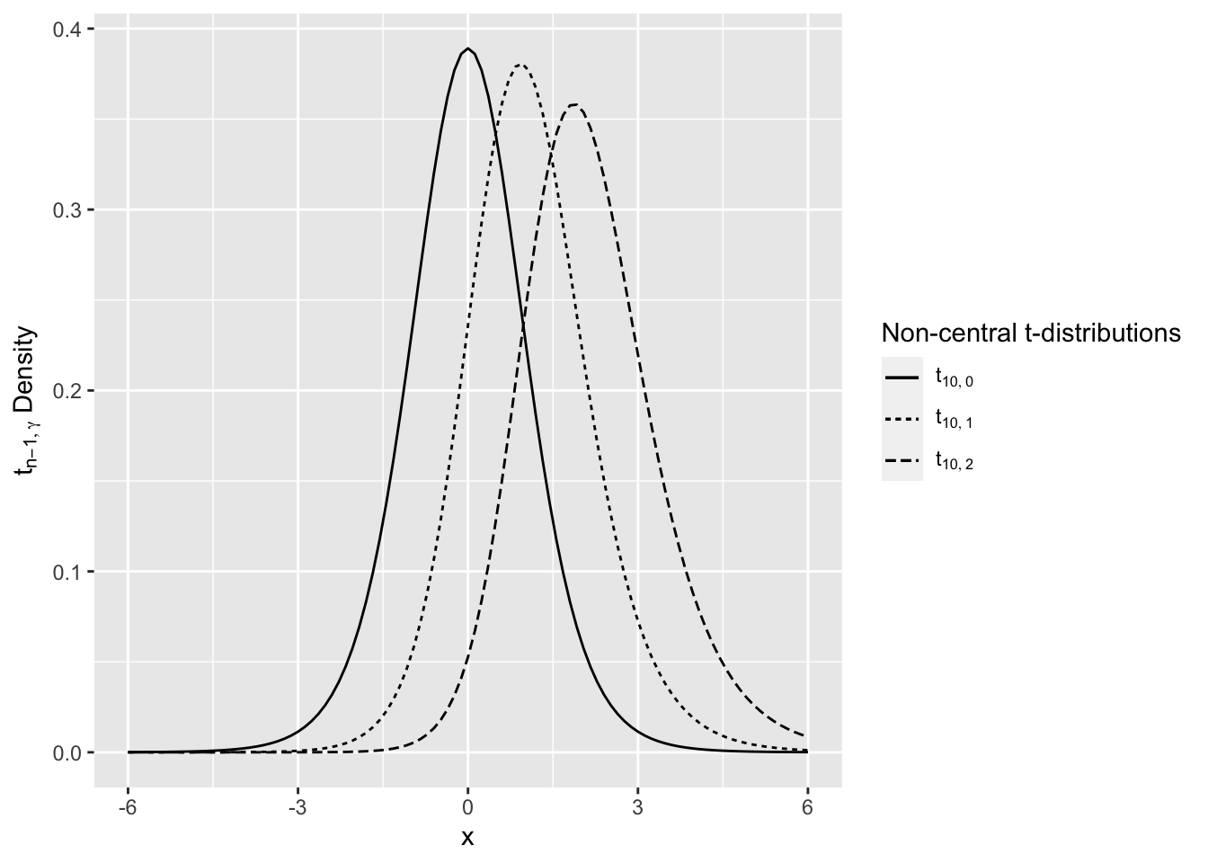
Figure 4.1: Noncentral t-distribution

The power of the test at \(\mu=\mu_1\) is

\[\begin{aligned} 1-\beta &= 1-P\left(\text{type II error}\right) \notag \\ &= P_{H_1}\left(\text{Reject } H_0\right) \notag\\ &= P_{H_1}\left(\text{Reject } H_0\right) \notag\\ &= P_{H_1}\left(\left|\frac {{\bar X} -\mu_0} {\frac{S}{\sqrt{n}}} \right| \ge t_{n-1, 1-\alpha/2}\right) \notag \\ &= P_{H_1}\left(\frac {{\bar X} -\mu_0} {\frac{S}{\sqrt{n}}} \ge t_{n-1, 1-\alpha/2}\right) + P_{H_1}\left(\frac {{\bar X} -\mu_0} {\frac{S}{\sqrt{n}}} < - t_{n-1, 1-\alpha/2}\right) \notag \\ &= P(t_{n-1,\gamma}\ge t_{n-1,1-\alpha/2})+P(t_{n-1,\gamma}< -t_{n-1,1-\alpha/2}). \end{aligned} \tag{4.2}\]

4.4.1 Computation Lab: Power of the One-Sample t-test

The following function calculates the power function using (4.2) for the one-sample t-test in R:

onesampttestpow <- function(alpha, n, mu0, mu1, sigma) {
  delta <- mu1 - mu0
  t.crit <- qt(1 - alpha / 2, n - 1)
  t.gamma <- sqrt(n) * (delta / sigma)
  t.power <-
    1 - pt(t.crit, n - 1, ncp = t.gamma) + 
    pt(-t.crit, n - 1, ncp = t.gamma)
  return(t.power)
}

Example 4.2 Calculate the power of \(H_0:\mu = 0 \mbox{ vs. } H_1:\mu = 0.15\) with \(n = 10\), \(\sigma = 0.2\), and \(\alpha = 0.05\) by calling the above function.

onesampttestpow(
  alpha = 0.05,
  n = 10,
  mu0 = 0,
  mu1 = 0.15,
  sigma = 0.2
)
#> [1] 0.5619533

This means that the test will reject \(H_0\) in 56.2% of studies testing this hypothesis (i.e., the study testing this hypothesis was replicated a large number of times).

stats::power.t.test() is part of the default R packages. Using this function on the previous example we get

power.t.test(
  n = 10,
  delta = 0.15,
  sd = 0.2,
  sig.level = 0.05,
  type = "one.sample"
)
#> 
#>      One-sample t test power calculation 
#> 
#>               n = 10
#>           delta = 0.15
#>              sd = 0.2
#>       sig.level = 0.05
#>           power = 0.5619339
#>     alternative = two.sided

Exactly one of the parameters n, delta, power, sd, and sig.level must be passed as NULL, and that parameter is determined from the others. In this example, the function calculates power given the other parameters. If sample size is required for, say, 80% power then use

power.t.test(
  power = 0.8,
  delta = 0.15,
  sd = 0.2,
  sig.level = 0.05,
  type = "one.sample"
)
#> 
#>      One-sample t test power calculation 
#> 
#>               n = 15.98026
#>           delta = 0.15
#>              sd = 0.2
#>       sig.level = 0.05
#>           power = 0.8
#>     alternative = two.sided

The calculation shows that a study testing \(H_0:\mu=\mu_0 \mbox{ vs } H_1:\mu=\mu_1\), where delta= \(\mu_0-\mu_1\) requires sixteen experimental units for 80% power.

4.5 Power of the Two-Sample t-test

The two-sample t-test, described in Section 3.9, is often used to test if the difference between two means is zero. This section develops the power of this test using the same notation as Section 3.9.

Recall from Section 3.9 that \(T_n\) is the two-sample t-statistic, where \(T_n \sim t_{n_1+n_2-2}\) under \(H_0\) and \(t_{n_1+n_2-2,\gamma}\) with non-centrality parameter \(\gamma ={\theta}/{\sigma\sqrt{1/n_1+1/n_2}},\) under \(H_1\).

\(H_0\) is rejected if \(\left| T_n \right| \ge t_{n_1+n_2-2,1-\alpha/2}\) where \(t_{\lambda,p}\) is the \(pth\) quantile of the central t-distribution with \(\lambda\) degrees of freedom.

The sample size can be determined by specifying the type I and type II error rates, the standard deviation, and the difference in treatment means that the study aims to detect.

In a derivation similar to the power of the one-sample t-test in Section 4.4, the power of the two-sample t-test is

\[1-\beta = P(t_{n_1+n_2-2, \gamma} \ge t_{n_1+n_2-2,\gamma ,1-\alpha/2})+P(t_{n_1+n_2-2, \gamma} < -t_{n_1+n_2-2,\gamma , 1-\alpha/2}),\]

where \(t_{\lambda,\gamma ,p}\) is the \(pth\) quantile of the non-central t-distribution with non-centrality parameter \(\gamma\) and \(\lambda\) degrees of freedom. The power is not a closed form expression so it’s not possible to derive a formula for the study sample size. Nevertheless, if the variance is assumed to be known, and if \(n_1=n_2=n/2,\) then the total sample size for a study at level \(\alpha\), power \(1-\beta\), that tests \(H_0:\theta=\theta_0 \mbox{ vs. } H_1:\theta = \theta_1\) is

\[\begin{equation} n=\frac{4\sigma^2\left(z_{1-\alpha/2}+z_{1-\beta}\right)}{\theta_1^2}. \tag{4.3} \end{equation}\]

4.5.1 Effect Size

In some studies, instead of specifying the difference in treatment means and standard deviation separately, the ratio

\[\text{ES} = \frac{\mu_1-\mu_2}{\sigma}\]

can be specified. This ratio is called the scaled effect size. Jacob Cohen³⁶ suggests that effect sizes of 0.2, 0.5, and 0.8 correspond to small, medium, and large effects.

4.5.2 Sample Size—Known Variance and Equal Allocation

Consider a study where experimental units are randomized into two treatment groups and the investigator would like an equal number of experimental units in each group.

If the variance is known, then a test statistic for testing if the means of two populations are equal is

\[ Z=\frac {{\bar Y}_1 - {\bar Y}_2}{\sigma \sqrt{(1/n_1+1/n_2)}} \sim N(0,1).\]

This is known as the two-sample z-test.

The power at \(\theta=\theta_1\) is given by

\[\begin{equation} 1-\beta = P\left( Z \ge z_{1-\alpha/2} - \frac{\theta_1}{\sigma \sqrt{1/n_1+1/n_2}} \right) \\ + P\left( Z < -z_{1-\alpha/2} - \frac{\theta_1}{\sigma \sqrt{1/n_1+1/n_2}} \right). \tag{4.4} \end{equation}\]

Ignoring terms smaller than \(\alpha/2\) and combining positive and negative \(\theta\) in (4.4)

\[\begin{equation} \beta \approx \Phi\left( z_{1-\alpha/2} - \frac{\left|\theta_1\right|}{\sigma \sqrt{1/n_1+1/n_2}} \right). \tag{4.5} \end{equation}\]

Applying \(\Phi^{-1}\) to (4.5) and using 2.1, it follows that

\[\begin{equation} z_{1-\beta}+z_{1-\alpha/2} = \left( \frac{\left|\theta_1\right|}{\sigma \sqrt{1/n_1+1/n_2}} \right). \tag{4.6} \end{equation}\]

If we assume that there will be an equal allocation of subjects to each group, then \(n_1 = n_2 = n/2\), and the total sample size is

\[\begin{equation} n= \frac {4\sigma^2 \left(z_{1-\beta}+z_{1-\alpha/2}\right)^2}{\theta^2}, \tag{4.7} \end{equation}\]

where \(\alpha, \beta \in (0,1).\)

4.5.3 Sample Size—Known Variance and Unequal Allocation

In many studies comparing two treatments, it is desirable to put more experimental units into the experimental group to learn more about this treatment. If the allocation of experimental units between the two groups is \(r = n_1/n_2\) then \(n_1 = r\cdot n_2\). Plugging this into (4.6) the sample size for \(n_2\) is

\[\begin{equation} n_2=\frac {(1+1/r)\sigma^2 \left(z_{\beta}+z_{\alpha/2}\right)^2} {\theta^2}. \tag{4.8} \end{equation}\]

4.5.4 Computation Lab: Power of the Two-Sample t-test

The following R function uses qt() to compute \(t_{n,\gamma,\lambda}\) and pt() to compute the \(t_{n,\gamma}\) CDF.

twosampttestpow <- function(alpha, n1, n2, mu1, mu2, sigma) {
  delta <- mu1 - mu2
  t.crit <- qt(1 - alpha / 2, n1 + n2 - 2)
  t.gamma <- delta / (sigma * sqrt(1 / n1 + 1 / n2))
  t.power <-
    (1 - pt(t.crit, n1 + n2 - 2, ncp = t.gamma) +
       pt(-t.crit, n1 + n2 - 2, ncp = t.gamma))
  return(t.power)
}

The power of a study to detect \(\theta = 1\) with \(\sigma = 3,n_1 = n_2 = 50\) is

twosampttestpow(
  alpha = .05,
  n1 = 50,
  n2 = 50,
  mu1 = 1,
  mu2 = 2,
  sigma = 3
)
#> [1] 0.3785749

stats::power.t.test() can also be used and gives the same results.

power.t.test(
  n = 50,
  delta = 1,
  sd = 3,
  sig.level = 0.05
)
#> 
#>      Two-sample t test power calculation 
#> 
#>               n = 50
#>           delta = 1
#>              sd = 3
#>       sig.level = 0.05
#>           power = 0.3784221
#>     alternative = two.sided
#> 
#> NOTE: n is number in *each* group

So the study would require 50 subjects per group to achieve 38% power to detect a difference of \(\theta = 1\) at the 5% significance level assuming \(\sigma = 3\). power.t.test() can also output the number of subjects required to achieve a certain power. Suppose the investigators want to know how many subjects per group would have to be enrolled in each group to achieve 80% power under the same conditions?

power.t.test(
  power = 0.8,
  delta = 1,
  sd = 3,
  sig.level = 0.05
)
#> 
#>      Two-sample t test power calculation 
#> 
#>               n = 142.2466
#>           delta = 1
#>              sd = 3
#>       sig.level = 0.05
#>           power = 0.8
#>     alternative = two.sided
#> 
#> NOTE: n is number in *each* group

142 subjects would be required in each group to achieve 80% power.

Figure 4.2 shows power of the two-sample t-test as a function of \(n\) and \(\theta\) (left), and \(n\) and \(\sigma\) (right) with a horizontal line drawn at 0.8 power for reference.

f <- function(n, d, sd)
  power.t.test(
    n = n,
    delta = d,
    sd = sd,
    type = "two.sample",
    alternative = "two.sided",
    sig.level = 0.05
  )$power

p1 <-
  ggplot() +
  xlim(0, 3.0) +
  scale_y_continuous(breaks = seq(0, 1, by = 0.1)) +
  geom_function(fun = f,
                args = list(n = 30, sd = 1.5),
                aes(linetype = "N = 30")) +
  geom_function(fun = f,
                args = list(n = 20, sd = 1.5),
                aes(linetype = "N = 20")) +
  geom_function(fun = f,
                args = list(n = 10, sd = 1.5),
                aes(linetype = "N = 10")) +
  ylab("Power") +
  xlab(TeX("$\\theta$")) +
  geom_hline(yintercept = 0.8) +
  guides(linetype = guide_legend(title = "Sample size"))

p2 <-
  ggplot() +
  xlim(0.15, 3.0) +
  scale_y_continuous(breaks = seq(0, 1, by = 0.1)) +
  geom_function(fun = f,
                args = list(n = 30, d = 1),
                aes(linetype = "N = 30")) +
  geom_function(fun = f,
                args = list(n = 20, d = 1),
                aes(linetype = "N = 20")) +
  geom_function(fun = f,
                args = list(n = 10, d = 1),
                aes(linetype = "N = 10")) +
  ylab("Power") +
  xlab(TeX("$\\sigma$")) +
  geom_hline(yintercept = 0.8) +
  guides(linetype = guide_legend(title = "Sample size"))

p1 + p2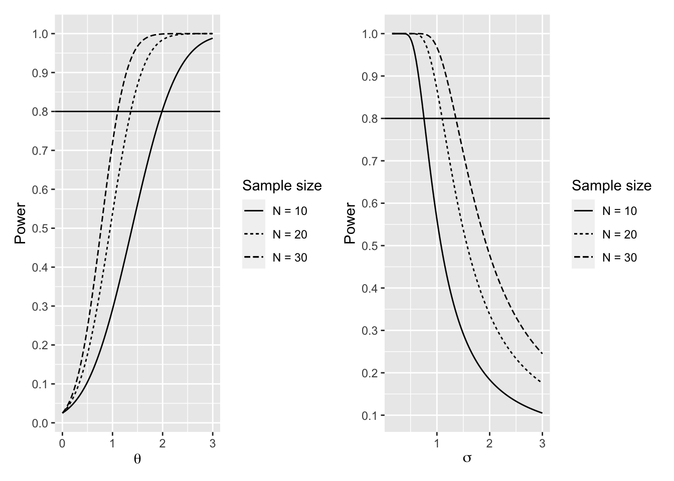

Figure 4.2: Power of Two-Sample t-test

Power as a function of effect size can be investigated by rearranging (4.4). In the R function below we assume \(n_1=n_2=10, ]\alpha=0.05\).

pow.t <- function(ES) {
  alpha <- 0.05
  nA <- 10
  nB <- 10
  t.crit <- qt(1 - alpha / 2, nA + nB - 2)
  t.gamma <- ES / (sqrt(1 / nA + 1 / nB))
  t.power <- (1 - pt(t.crit, nA + nB - 2, ncp = t.gamma) +
                pt(-t.crit, nA + nB - 2, ncp = t.gamma))
  t.power
}

The code below was used to create Figure 4.3.

ggplot() +
  scale_x_continuous(limits = c(-2, 2), 
                     breaks = seq(-2, 2, by = 0.5)) +
  scale_y_continuous(limits = c(0, 1), 
                     breaks = seq(0, 1, by = 0.1)) +
  geom_function(fun = pow.t) +
  ylab("Power") +
  xlab("Effect Size")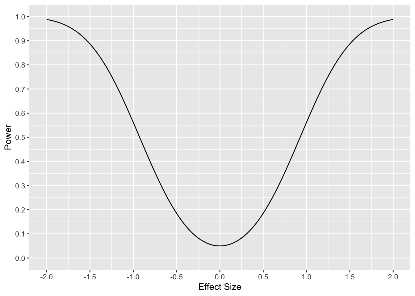

Figure 4.3: Two-Sample t-test Power and Effect Size, N = 10

The R code below defines a function to compute the sample size in groups 1 and 2 for unequal allocation using (4.8).

size2z.uneq.test <- function(theta, alpha, beta, sigma, r)
{
  zalpha <- qnorm(1 - alpha / 2)
  zbeta <- qnorm(1 - beta)
  n2 <- (1 + 1 / r) * (sigma * (zalpha + zbeta) / theta) ^ 2
  n1 <- r * n2
  c(n1, n2)
}

The number of patients in group 1 is computed using size2z.uneq.test.

# sample size for theta =1, alpha = 0.05, 
# beta = 0.1, sigma = 2, r = 2

size2z.uneq.test(
  theta = 1,
  alpha = .05,
  beta = .1,
  sigma = 2,
  r = 2
)[1] # group 1 sample size (experimental group)
#> [1] 126.0891

So, the number of patients in the experimental group is 126. The number in the control group is computed below.

size2z.uneq.test(
  theta = 1,
  alpha = .05,
  beta = .1,
  sigma = 2,
  r = 2
)[2] # group 2 sample size (control group)
#> [1] 63.04454

The sample size required for 90% power to detect \(\theta = 1\) with \(\sigma = 2\) at the 5% level in a trial where two patients will be enrolled in the experimental arm for every patient enrolled in the control arm is 126 in the control group and 63 in the experimental group. The total sample size is 189.

The power of the two-sample z-test (4.5) can be studied as a function of the allocation ratio \(r\). The code chunk below produces Figure 4.4.

# power of z test as a function of allocation ratio r,
# total sample size n, alpha, theta, and sigma
pow_ztest <- function(r, n, alpha, theta, sigma)
{
  n2 <- n / (r + 1)
  x <- qnorm(1 - alpha / 2) - abs(theta) / 
    (sigma * sqrt(1 / (r * n2) + 1 / n2))
  pow <- 1 - pnorm(x)
  return(pow)
}

ggplot() + xlim(0.1, 5) +
  geom_function(
    fun = pow_ztest,
    args = list(
      n = 25,
      alpha = 0.05,
      theta = 1,
      sigma = 1
    ),
    aes(linetype = "N = 25")
  ) +
  geom_function(
    fun = pow_ztest,
    args = list(
      n = 50,
      alpha = 0.05,
      theta = 1,
      sigma = 1
    ),
    aes(linetype = "N = 50")
  ) +
  ylab("Power") + xlab(TeX("$\\r$")) +
  guides(linetype = guide_legend(title = "Allocation ratio"))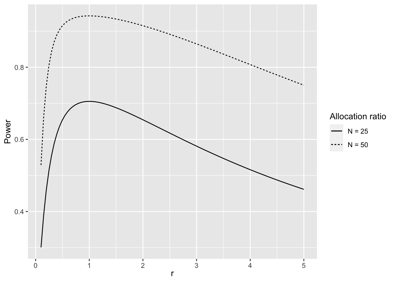

Figure 4.4: Power of z-test as a Function of Allocation Ratio and Sample Size

As the allocation ratio increases the power decreases assuming other parameters remain fixed (see Figure 4.4).

4.6 Power and Sample Size for Comparing Proportions

This section discusses power and sample size for studies where the primary study outcomes are dichotomous.

Let \(p_1\) denote the response rate in group 1, \(p_2\) the response rate in group 2, and let the difference be \(\theta= p_1—p_2\). A binary outcome for subject \(i\) in arm \(k\) is

\[Y_{ik} = \left\{ \begin{array}{ll} 1 & \mbox{with probability } p_k \\ 0 & \mbox{with probability } 1-p_k, \end{array} \right.\]

for \(i = 1,...,n_k\) and \(k = 1,2\). The sum of independent and identically distributed Bernoulli random variables has a binomial distribution,

\[ \sum_{i = 1}^{n_k} Y_{ik} \sim Bin(n_k,p_k), \thinspace k = 1,2.\]

The sample proportion for group \(k\) is

\[{\hat p}_k= \frac{1}{n_k}\sum_{i = 1}^{n_k} Y_{ik}, \thinspace k = 1,2,\]

and \(E\left( {\hat p}_k\right)=p_k\) and \(Var\left({\hat p}_k \right)=p_k(1-p_k)/{n_k}\).

Consider a study where the aim is to determine if there is a difference between the two groups. That is we want to test \(H_0: \theta = 0\) versus \(H_1: \theta \ne 0.\)

If \(H_0\) is true then the test statistic

\[Z = \frac {{\hat p}_1-{\hat p}_2} {\sqrt{p_1(1-p_1)/n_1+p_2(1-p_2)/n_2}} \sim N(0,1).\]

The test rejects at level \(\alpha\) if and only if

\[\left|Z\right| \ge z_{1-\alpha/2}.\]

Using the same argument as the case with continuous endpoints in Section 4.5.2 and ignoring terms smaller than \(\alpha/2\), we can solve for \(\beta\)

\[\begin{equation} \beta \approx \Phi\left( z_{1-\alpha/2}- \frac{|\theta_1|}{\sqrt{p_1(1-p_1)/n_1+p_2(1-p_2)/n_2}}\right). \tag{4.9} \end{equation}\]

A formula for sample size can be derived using (4.9). If \(n_1 = r \cdot n_2\) then

\[n_2= \frac {\left(z_{1-\alpha/2}+z_{1-\beta}\right)^2}{\theta^2} \left(p_1(1-p_1)/r+p_2(1-p_2) \right),\] where \(\alpha,\beta \in (0,1).\)

4.6.1 Computation Lab: Power and Sample Size for Comparing Proportions

stats::power.prop.test() can be used to calculate sample size or power.

Example 4.3 The standard treatment for a disease has a response rate of 20%, and an experimental treatment is anticipated to have a response rate of 28%. The investigators want both groups to have an equal number of subjects. How many patients should be enrolled if the study will conduct a two-sided test at the 5% level with 80% power?

power.prop.test(p1 = 0.2, p2 = 0.28, power = 0.8)
#> 
#>      Two-sample comparison of proportions power calculation 
#> 
#>               n = 446.2054
#>              p1 = 0.2
#>              p2 = 0.28
#>       sig.level = 0.05
#>           power = 0.8
#>     alternative = two.sided
#> 
#> NOTE: n is number in *each* group

This means that 446 patients should be enrolled in each group for a study to have a power of 0.8 to detect \(p_1=0.2\) and \(p_2=0.28\) at the \(\alpha=0.05\) level.

4.7 Calculating Power by Simulation

Statistical power is the probability that the test correctly rejects the null hypothesis. Consider a thought experiment: imagine being able to replicate a study with different random samples a large number of times, and each time the null hypothesis is tested. If the null hypothesis is false, it’s reasonable to expect a large proportion of these tests reject the null hypothesis. This thought experiment can be operationalized via simulation.

4.7.1 Algorithm for Simulating Power

Use an underlying model to generate random data with (a) specified sample sizes, (b) parameter values that are being tested via the hypothesis test, and (c) other (nuisance) parameters such as variances.
Run an estimation program (e.g., a two-sample t-test) on these randomly generated data.
Calculate the test statistic and p-value.
Repeat steps 1–3 many times, say, N, and save the p-values. The estimated power for a level alpha test is the proportion of observations (out of N) for which the p-value is less than alpha.

4.7.2 Computation Lab: Simulating Power of a Two-Sample t-test

If the test statistic and distribution of the test statistic are known, then the power of the test can be calculated via simulation.

Example 4.4 Consider a two-sample t-test with 30 subjects per group and the standard deviation known to be 1. What is the power of the test \(H_0:\mu_1-\mu_2 = 0\) versus \(H_1:\mu_1-\mu_2 = 0.5\), at the 5% significance level?

Power is the proportion of times that the test correctly rejects the null hypothesis in repeated testing of the same hypothesis based on different randomly drawn samples.

A single study is simulated below. Let’s assume that \(n_1 = n_2 = 30\), \(\mu_1 = 3.5\), \(\mu_2 = 3\), \(\sigma = 1\), and \(\alpha = 0.05\).

set.seed(2301)

samp1 <- rnorm(30, mean = 3.5, sd = 1)
samp2 <- rnorm(30, mean = 3, sd = 1)

twosampt <- t.test(samp1, samp2, var.equal = T)
twosampt$p.value
#> [1] 0.03604893

The null hypothesis would be rejected at the 5% level.

Suppose that 10 studies are simulated. What proportion of these 10 studies will reject the null hypothesis at the 5% level? To investigate how many times the two-sample t-test will reject at the 5% level, the replicate() function will be used to generate 10 studies and calculate the p-value in each study. It will still be assumed that \(n_1 = n_2 = 30\), \(\mu_1 = 3.5\), \(\mu_2 = 3\), \(\sigma = 1\), and \(\alpha = 0.05\).

set.seed(2301)

tpval <- function() {
  n <- 30
  mu1 <- 3.5
  mu2 <- 3.0
  sigma <- 1
  samp1 <- rnorm(n, mean = mu1, sd = sigma)
  samp2 <- rnorm(n, mean = mu2, sd = sigma)
  twosamp <- t.test(samp1, samp2, var.equal = T)
  return(twosamp$p.value)
}

reps <- 10

pvals <- replicate(reps, tpval())
#power is the number of times the test rejects at the 5% level
sum(pvals <= 0.05) / reps 
#> [1] 0.3

But, since we only simulated 10 studies the estimate of power will have a large standard error. So let’s try simulating 10,000 studies so that we can obtain a more precise estimate of power.

set.seed(2301)

reps <- 10000
pvals <- replicate(reps, tpval())
sum(pvals <= 0.05) / reps 
#> [1] 0.4881

This is much closer to the theoretical power obtained from stats::power.t.test().

powt <- power.t.test(
  n = 30,
  delta = 0.5,
  sd = 1,
  sig.level = 0.05
)
powt$power
#> [1] 0.477841

Example 4.5 Suppose that the standard treatment for a disease has a response rate of 20%, and an experimental treatment is anticipated to have a response rate of 28%. The researchers are considering enrolling 1,500 patients in the standard group and 500 patients in the experimental arm. What is the power of this study?

The number of subjects in the experimental arm that have a positive response to treatment will be an observation from a \(Bin(1500,0.20)\) and the number of subjects that have a positive response to the standard treatment will be an observation from a \(Bin(500,0.28)\). We can obtain simulated responses from these distributions using the rbinom() function.

set.seed(2301)
rbinom(1, 500, 0.28)
#> [1] 132
rbinom(1, 1500, 0.20)
#> [1] 324

In this simulated study, 132 of the 500 patients in the experimental arm had a positive response to the experimental treatment and 324 of the 1,500 patients in the control arm had a positive response to the standard treatment. The p-value for this simulated study can be obtained using prop.test().

set.seed(2301)

samp1 <- rbinom(1, 500, 0.28) 
samp2 <- rbinom(1, 1500, 0.20)

twosamp <- prop.test(
  x = c(samp1, samp2),
  n = c(500, 1500),
  correct = F
)

twosamp$p.value
#> [1] 0.0267226

In this study, the p-value is 0.03, which is less than 0.05 so there would be evidence that the new treatment is significantly better than the standard treatment. A power simulation repeats this process a large number of times. The replicate() command can be used for the repetition.

set.seed(2301)

proppval <- function() {
  n1 <- 500
  p1 <- 0.28
  n2 <- 1500
  p2 <- 0.20
  samp1 <- rbinom(n = 1, size = n1, prob = p1)
  samp2 <- rbinom(n = 1, size = n2, prob = p2)
  twosamp <- prop.test(x = c(samp1, samp2),
                       n = c(n1, n2),
                       correct = F)
  return(twosamp$p.value)
}

reps <- 10000
pvals <- replicate(reps, proppval())
sum(pvals <= 0.05) /  reps
#> [1] 0.9534

The power of the study in this case is 0.95.

4.8 Exercises

Exercise 4.1 Consider the power function of one-sample z-test shown in Equation (4.1). What is the limit of the power function as \(n \rightarrow \infty\)? How about when \(\mu_1\rightarrow \mu_0\)? What do the results tell you about the power of the one-sample z-test?

Exercise 4.2 Show that

\[\begin{aligned} & P_{H_1}\left(\frac {{\bar X} -\mu_0} {\frac{S}{\sqrt{n}}} \ge t_{n-1, 1-\alpha/2}\right) + P_{H_1}\left(\frac {{\bar X} -\mu_0} {\frac{S}{\sqrt{n}}} < - t_{n-1, 1-\alpha/2}\right) \notag \\ =& P(t_{n-1,\gamma}\ge t_{n-1,1-\alpha/2})+P(t_{n-1,\gamma}< -t_{n-1,1-\alpha/2}). \end{aligned}\]

The right-hand side is the final expression for the power of the t-test in Section 4.4.

Exercise 4.3 Derive equation (4.3) for the total sample of the two-sample t-test.

Exercise 4.4 Consider the derivation of Equation (4.7) for the sample size of a two-sample z-test with known variance and equal allocation.

Identify terms in Equation (4.4) that are smaller than \(\alpha/2\) and derive line (4.5) based on the information.
Show how Equation (4.6) is derived from Equation (4.5).

Exercise 4.5 Consider Figure 4.2 and the R code that generated the plots.

Modify the code so that sample size is on the x-axis, and three different lines show the relationships between sample size and power for a difference of \(\theta=1,2,3\). Fix the standard deviation to 1.5 for all lines.
Interpret the relationships between power, effect size \(\theta\), standard deviation \(\sigma\), and sample size \(n\), on Figure 4.2 and the figure from part a. For example, what happens to power as \(\theta\) decreases with \(n\) and \(\sigma\) fixed? How does \(\theta\) change as power increases with other parameters fixed?

Exercise 4.6 Consider the plot of power as a function of effect size for the two-sample t-test shown in Figure 4.3.

Create a plot to show power as a function of both effect size and sample size while keeping other parameters fixed.
The curve is shaped like an inverted bell curve, or a “bathtub” shape. Interpret the shape of the curve.

Exercise 4.7 Consider the plot of power as a function of the allocation ratio, \(r\), for the two-sample z-test shown in Figure 4.4 and the R code for generating plot.

Recall that n is the total sample size for the function pow_ztest(). What does n2 represent, and why is it n/(r+1)?
Does sample size imbalance between the two groups lead to an increase or decrease in power? Explain.
Modify the function pow_ztest() to return the value of n2 and plot n2 versus r. Describe the relationship between the two variables.

Exercise 4.8 The R function size2z.test() shown below implements the sample size formula for calculating the sample size for a test of \(H_0:\theta = 0\) versus \(H_1: \theta \ne 0\), where \(\theta=\mu_1-\mu_2\).

size2z.test <- function(theta, alpha, beta, sigma)
{
  zalpha <- qnorm(1-alpha/2)
  zbeta <- qnorm(1-beta)
  (2*sigma*(zalpha+zbeta)/theta)^2
}

What are the main assumptions behind this sample size formula?
Assuming all other parameters remain fixed, indicate whether the sample size increases or decreases in each of the following cases.
1. As \(\sigma\) decreases.
2. As \(\alpha\) decreases.
3. As \(\theta\) decreases.

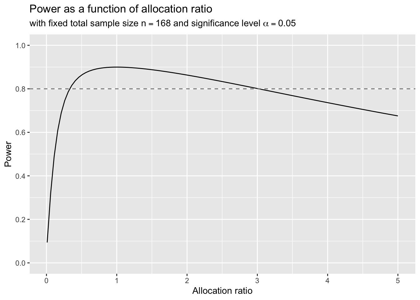
Exercise 4.9 A statistician is designing a phase III clinical trial comparing a continuous outcome in two groups receiving experimental versus standard therapy with a total sample size of 168 patients. The team requires the study have 80% power at the 5% significance level to detect a difference of 1. Assume that the standard deviation of the outcome is 2. The design team would like to investigate whether it’s possible to have four times as many patients in the experimental group versus the control group without having to increase the total sample size.

What is the power if there are four times as many patients in the experimental group? What should the statistician recommend to the team in order for the study to have at least 80% power?

Exercise 4.10 Let \(X_1, X_2, ..., X_n\) be iid \(N\left(\mu,\sigma^2\right)\).

Show that the power function of the test \(H_0:\mu = 0\) versus \(H_1:\mu > 0\) at \(\mu=1\) is

\[1-\Phi\left(z_{\frac{\alpha}{2}}-\frac{\sqrt{n}}{\sigma}\right),\]

where \(z_{\frac{\alpha}{2}}\) is the \(100\left(1-\frac{\alpha}{2}\right)^{th}\) percentile of the \(N\left(0,1\right)\).
Use R to calculate the power when \(n = 10\), \(\alpha = 0.01\), and \(\sigma = 1\).

3 Comparing Two Treatments

5 Comparing More Than Two Treatments