6 Factorial Designs at Two Levels—\(2^k\) Designs
6.1 Introduction
A factorial design is an experimental design where the investigator selects a fixed number of factors with \(k\ge2\) levels and then measures response variables at each factor-level combination. The factors can be quantitative or qualitative. For example, two levels of a quantitative variable could be two different temperatures or two different concentrations. Qualitative factors might be two types of catalysts or the presence and absence of some entity.
A \(2^k\) factorial design is notation for a factorial design where:
the number of factors is \(k\ge 2\),
the number of levels of each factor is 2, and
the total number of experimental conditions, called runs, in the design is \(2^k\).
In general, factorial experiments can involve factors with different numbers of levels. For example, a factorial experiment that involves three factors with three levels and two factors with two levels would be a \(3^3 \times2^2\) design.
Example 6.1 An investigator is interested in examining three components of a weight loss intervention.
A. Keeping a food diary
B. Increasing activity
C. Home visit
The investigator plans to investigate all \(2 \times 2 \times 2 = 2^3= 8\) combinations of experimental conditions.
The experimental conditions are outlined in Table ??. The notation \((-, +)\) is often used to represent the two factor levels in a \(2^k\) design. In this case, \(-\) represents No and \(+\) represents Yes. The response variable for the \(i^{th}\) run (\(i=1,\ldots,8\)) is represented by \(y_i\), and the observed value is recorded in brackets next to \(y_i\).
6.2 Factorial Effects
In ANOVA, the objective is to compare the individual experimental conditions with each other. In a factorial experiment, the objective is generally to compare combinations of experimental conditions.
What is the effect of keeping a food diary in Example 6.1?
6.2.1 Main Effects
We can estimate the effect of a food diary by comparing the mean of all conditions where food diary is set to NO (Run 1-4) and the mean of all conditions where food diary is set to YES (Run 5-8) (see Table ??). This is also called the main effect of food diary, the adjective main being a reminder that this average is taken over the levels of the other factors.
Let \(\bar y(A+)\) be the average of the \(y\) values at the \(+\) level of A, and \(\bar y(A-)\) be the average of the \(y\) values at the \(-\) levels of A.
The main effect of food diary, \(ME(A)\), is
\[\begin{aligned} ME(A) = \bar y(A+) - \bar y(A-) &= \frac{y_1+y_2+y_3+y_4}{4}-\frac{y_5+y_6+y_7+y_8}{4} \\ &= \frac{1.1+1.8-0.3-1.1}{4} + \frac{1.0+2.6-0.4+0.4}{4}\\ &= 0.525. \end{aligned}\]
Similarly, the main effects of physical activity (B) and home visit (C) are:
\[\begin{aligned} ME(B) &= \bar y(B+) - \bar y(B-) = \frac{y_1+y_2+y_5+y_6}{4}-\frac{y_3+y_4+y_7+y_8}{4}=-1.975, \\ ME(C) &= \bar y(C+) - \bar y(C-) =\frac{y_1+y_3+y_5+y_7}{4}-\frac{y_2+y_4+y_6+y_8}{4}=0.575 \end{aligned}\]
Figure 6.1 shows a main effects plot for Example 6.1. The averages of all observations at each level of the factor are shown as dots connected by lines. The plot shows that keeping a food diary and a home visit increase weight loss, and increased physical activity decreases weight loss.
All experimental subjects are used, but are rearranged to make each comparison. In other words, subjects are recycled to measure different effects. This is one reason why factorial experiments are more efficient.
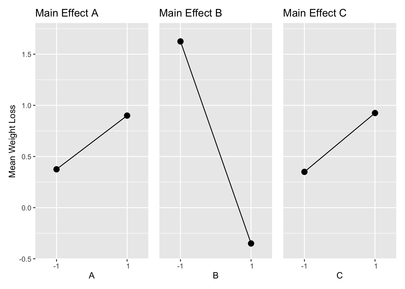
Figure 6.1: Main Effects of Example 6.1
6.2.2 Interaction Effects
Let \(\bar y(A+|B-)\) be the average of \(y\) at the \(+\) level of A when B is at the \(-\) level. The conditional main effect of A at the \(+\) level of B is then \(ME(A|B+) = \bar y(A+|B+) - \bar y(A-|B+)\). AB and ABC will be used for notation for the interaction between factors A and B, and A, B, and C.
6.2.2.1 Two Factor Interactions
The effect of food diary when home visit is No is
\[\begin{aligned} ME(A|B-) &=\bar y(A+|B-) - \bar y(A-|B-) \\ &= \frac{(y_5+y_6)}{2} - \frac{(y_1+y_2)}{2}\\ &= \frac{(1.0+2.6)}{2} -\frac{(1.1+1.8)}{2} \\ &= 0.35. \end{aligned}\] The effect of food diary when home visit is Yes is
\[\begin{aligned} ME(A|B+) &=\bar y(A+|B+) - \bar y(A-|B+) \\ &= \frac{(y_7+y_8)}{2} - \frac{(y_3+y_4)}{2} \\ &= \frac{((-0.4) + 0.4)}{2} - \frac{(-0.3 +(- 1.1))}{2} \\ &= 0.70. \end{aligned}\]
The average difference between \(ME(A|B-)\) and \(ME(A|B+)\) is the interaction between factors A and B
\[\begin{aligned} INT(A,B) &= \frac{1}{2}\left[ME(A|B+)-ME(A|B-)\right] \\ &= \frac{1}{2}[0.70-0.35] \\ &= 0.175. \end{aligned}\]
If there is a large difference between \(ME(A|B-)\) and \(ME(A|B+)\), then the effect of factor A may depend on the level of B. In this case, we say that there is an interaction between A and B.
The interaction between A and B from Example 6.1 is shown in Figure 6.2. This plot shows the means of \(y\) at each level of A and B. If the distance between ▲ and ● at each level of B is approximately the same, then the main effect of A doesn’t depend on the level of B. These plots can often be more informative than the single number of the interaction effect.
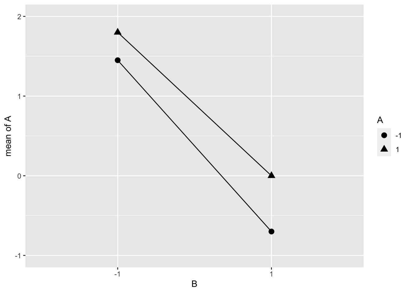
Figure 6.2: Interaction between Food Diary and Physical Activity (Example 6.1)
6.2.3 Three Factor Interactions
The interaction between food diary (A) and increased physical activity (B) in Example 6.1 when home visit (C) is No is \(INT(A,B|C-)\), and \(INT(A,B|C+)\) when home visit is Yes. The average difference between \(INT(A,B|C-)\) and \(INT(A,B|C+)\) is the three-way interaction between A, B, C or \(INT(A,B,C)\).
When C = 1 the interaction between A and B is
\[\begin{aligned} \frac{1}{2}\left[ME(A|B+,C+) - ME(A|B-,C+) \right] &= \frac{1}{2}\left[(y_8-y_4) - (y_6-y_2) \right] \\ &= \frac{1}{2}\left[(0.4-(-1.1)) - (2.6-1.8) \right] \\ &= 0.35. \end{aligned}\]
When C = -1 the interaction between A and B is
\[\begin{aligned} \frac{1}{2}\left[ME(A|B+,C-) - ME(A|B-,C-) \right] &= \frac{1}{2}\left[(y_7-y_3) - (y_5-y_1) \right] \\ &= \frac{1}{2}\left[(-0.4-(-0.3)) - (1.0-1.1) \right] \\ &= 0. \end{aligned}\]
Now, we take the average difference to get the three-factor interaction.
\[\begin{aligned} INT(A,B,C) &= \frac{1}{2}\left[INT(A,B|C+) - INT(A,B|C-)\right] \\ &= \frac{1}{2}[0.35-0] \\ &= 0.175. \end{aligned}\]
6.2.4 Cube Plot and Model Matrix
Figure 6.3 shows a cube plot for weight loss in Example 6.1. The cube plot shows the observations for each factor-level combination in a \(2^3\) design. The value of \(y\) for the various combinations of factors A, B, and C is shown at the corners of the cube. For example, \(y = 1.8\) was obtained when A = -1, B = -1, and C = 1. The cube shows how this design produces 12 comparisons along the 12 edges of the cube: four measures of the effect of food diary change; four measures of the effect of increased physical activity; four measures of home visit. On each edge of the cube, only one factor is changed with the other two held constant.
The same information is also displayed in the first three columns of the model matrix in Table 6.1. The first column has single -1 and 1 alternating, in the second pairs of -1 and 1 are alternating, etc. When a full factorial design matrix is specified in this manner the design is said to be in standard order. The interactions AB, AC, BC, ABC are the products of the columns A and B, A and C, etc.
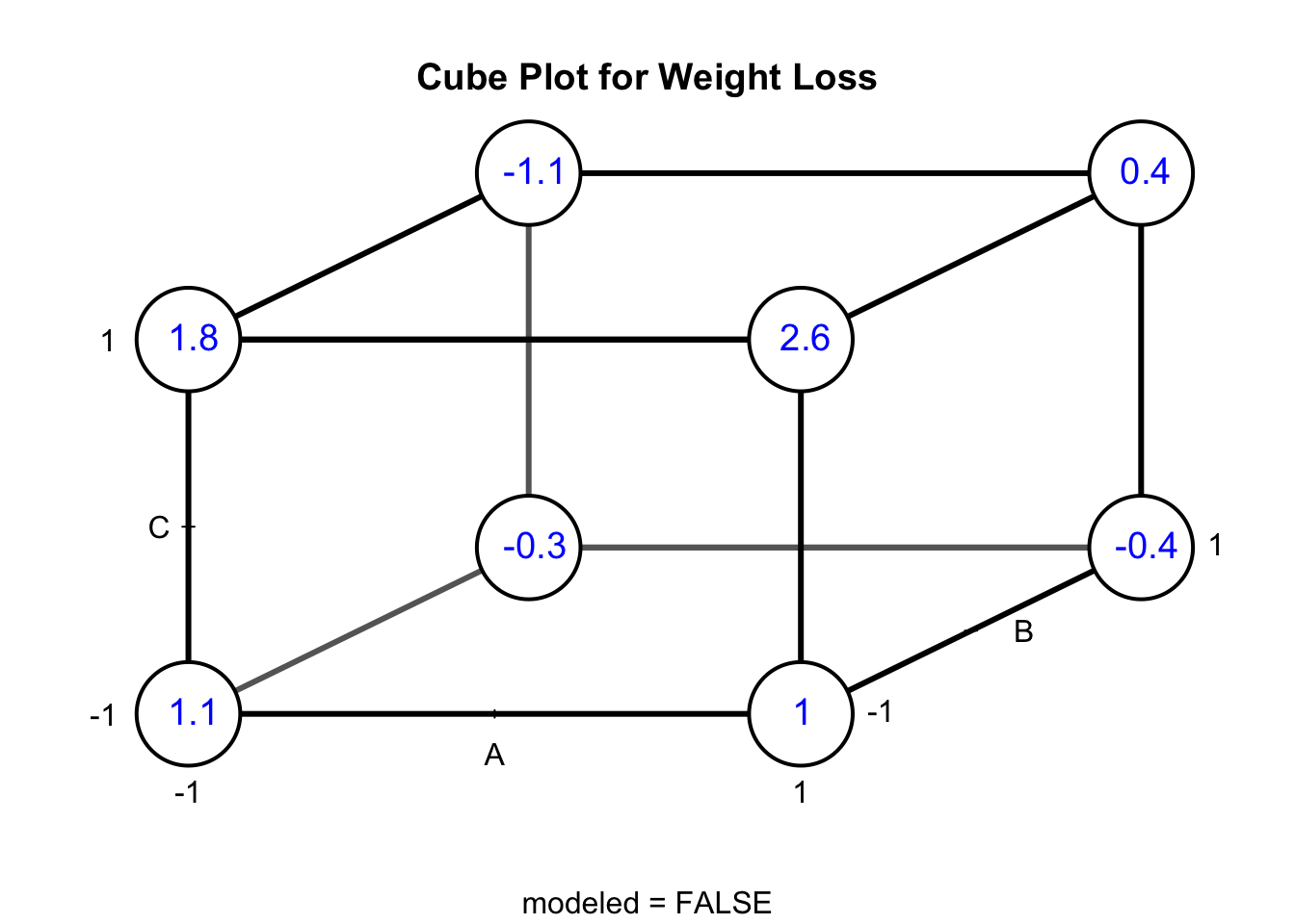
Figure 6.3: Cube Plot for Weight Loss from Example 6.1
| A | B | C | AB | AC | BC | ABC | y |
|---|---|---|---|---|---|---|---|
| -1 | -1 | -1 | 1 | 1 | 1 | -1 | 1.1 |
| -1 | -1 | 1 | 1 | -1 | -1 | 1 | 1.8 |
| -1 | 1 | -1 | -1 | 1 | -1 | 1 | -0.3 |
| -1 | 1 | 1 | -1 | -1 | 1 | -1 | -1.1 |
| 1 | -1 | -1 | -1 | -1 | 1 | 1 | 1.0 |
| 1 | -1 | 1 | -1 | 1 | -1 | -1 | 2.6 |
| 1 | 1 | -1 | 1 | -1 | -1 | -1 | -0.4 |
| 1 | 1 | 1 | 1 | 1 | 1 | 1 | 0.4 |
The model matrix can be be used to calculate factorial effects. For example, the main effect for B can be calculated by multiplying the B column and y column in Table 6.1 and dividing by 4.
6.2.5 Computation Lab: Computing and Plotting Factorial Effects
In this section we will use R to compute factorial effects for the data in Example 6.1. The data are stored in the data frame wtlossdat.
glimpse(wtlossdat, n = 3)
#> Rows: 8
#> Columns: 5
#> $ A           <dbl> -1, -1, -1, -1, 1, 1, 1, 1
#> $ B           <dbl> -1, -1, 1, 1, -1, -1, 1, 1
#> $ C           <dbl> -1, 1, -1, 1, -1, 1, -1, 1
#> $ y           <dbl> 1.1, 1.8, -0.3, -1.1, 1.0, 2.6, -0.4, …
#> $ `Run Order` <dbl> 5, 8, 1, 2, 4, 7, 3, 6
The main effect of a factor is the mean difference when a factor is at its high versus low level. The main effect of factor A is \(\bar y(A+)-\bar y(A-)\).
wtlossdat["y"] selects the column y from wtlossdat data frame.
Let’s write a function to compute the main effect to avoid copying and pasting similar code for each factor. The function takes a data frame (df), dependent variable (y1), and factor (fct1) that we want to calculate the main effect.
calcmaineff <- function(df, y1, fct1) {
  mean(df[y1][df[fct1] == 1]) - mean(df[y1][df[fct1] == -1])
}
We can use the function to calculate the main effects of B and C.
calcmaineff(df = wtlossdat, y1 = "y", fct1 = "B")
#> [1] -1.975
calcmaineff(df = wtlossdat, y1 = "y", fct1 = "C")
#> [1] 0.575
Another method to calculate factorial effects is to use the design matrix. For example, the main effect of C is the dot product of the C column and the y column divided by 4.
sum(wtlossdat["C"] * wtlossdat["y"]) / 4
#> [1] 0.575
Figure 6.4 uses ggplot() to plot the main effects.
wtlossdat %>%
  group_by(A) %>%
  summarise(mean = mean(y)) %>%
  ggplot(aes(A, mean)) +
  geom_point(size = 3) + geom_line() +
  ggtitle("Main Effect A") +
  ylab("Mean Weight Loss") +
  scale_x_discrete(limits = c(-1, 1))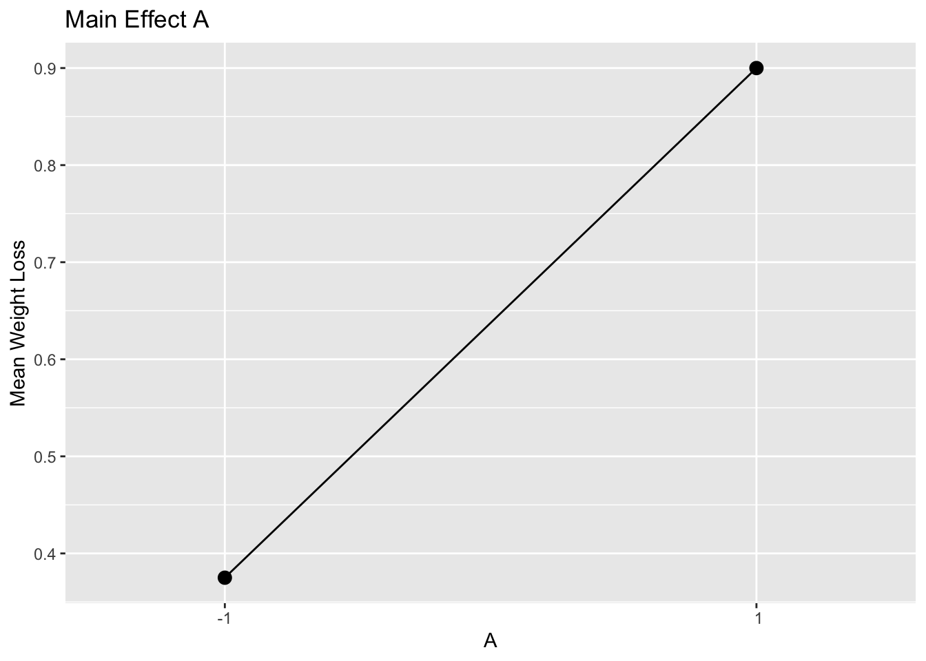
Figure 6.4: Main Effect of A Example 6.1
The two factor interaction between A and B is calculated by the following
- Compute the mean difference between (i)
ywhenA == 1andB == 1; and (ii)ywhenA == -1andB == 1. - Compute the mean difference between (i)
ywhenA == 1andB == -1; and (ii)ywhenA == -1andB == -1. - Compute the mean difference between 1. and 2.
# 1.
abplus <-
  (mean(wtlossdat$y[(wtlossdat$A == 1 & wtlossdat$B == 1)]) -
     mean(wtlossdat$y[(wtlossdat$A == -1 & wtlossdat$B == 1)]))
# 2.
abminus <-
  (mean(wtlossdat$y[(wtlossdat$A == 1 & wtlossdat$B == -1)]) -
     mean(wtlossdat$y[(wtlossdat$A == -1 & wtlossdat$B == -1)]))
# 3.
(abplus - abminus) / 2
#> [1] 0.175
We can also modify the function we wrote to compute main effects for two-way interactions.
calcInteract2 <- function(df, y1, fct1, fct2) {
  yzplus <- mean(df[y1][df[fct1] == 1 & df[fct2] == 1]) -
    mean(df[y1][df[fct1] == -1 & df[fct2] == 1])

  yzminus <- mean(df[y1][df[fct1] == 1 & df[fct2] == -1]) -
    mean(df[y1][df[fct1] == -1 & df[fct2] == -1])

  return(0.5 * (yzplus - yzminus))
}
The three two-way interactions are:
calcInteract2(wtlossdat, "y", "A", "B")
#> [1] 0.175
calcInteract2(wtlossdat, "y", "A", "C")
#> [1] 0.625
calcInteract2(wtlossdat, "y", "B", "C")
#> [1] -0.575
Interactions can also be calculated using the design matrix. For example, the BC interaction is the dot product of columns B, C, and y divided by 4.
sum(wtlossdat["B"] * wtlossdat["C"] * wtlossdat["y"]) / 4
#> [1] -0.575
Figure 6.5 shows an interaction plot of the AB interaction using interaction.plot().
interaction.plot(
  wtlossdat$B,
  wtlossdat$A,
  wtlossdat$y,
  trace.label = "A",
  xlab = "B",
  ylab = "Mean weight loss"
)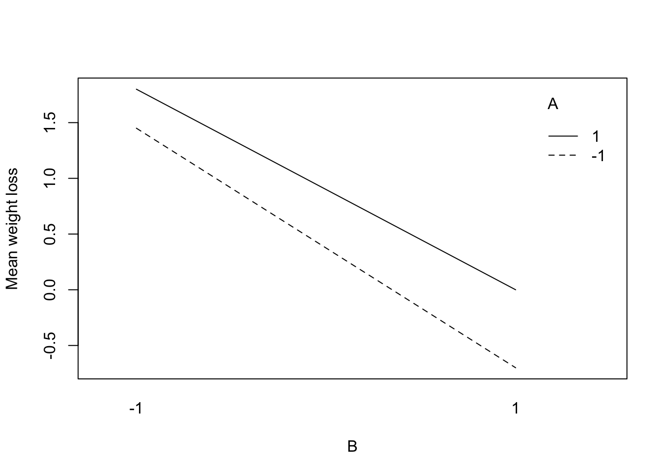
Figure 6.5: AB Interaction for Example 6.1
The code below uses ggplot() to create an interaction plot similar to Figure 6.5, although there is an extra step where the means are computed and stored in a data frame.
wtlossdat %>%
  group_by(A, B) %>%
  summarise(mean = mean(y)) %>%
  ggplot(aes(as.factor(B), mean, group = A)) +
  ylim(-1, 2) +
  geom_line(aes(linetype = as.factor(A))) +
  xlab("B") +
  ylab("mean of A") +
  guides(linetype = guide_legend(title = "A"))
Cube plots can be created using FrF2::cubePlot(). A simple way to use cubePlot() is to input a linear model object of the factorial design (discussed in Section 6.4). The modeled = FALSE argument indicates that we want to show the averages instead of the model means. The code below was used to create Figure 6.3.
mod <- lm(y ~ A * B * C, data = wtlossdat)
FrF2::cubePlot(
  mod,
  eff1 = 'A',
  eff2 = 'B',
  eff3 = 'C',
  main = "Cube Plot for Weight Loss",
  round = 2,
  modeled = F,
  cex.title = 1
)
6.3 Replication in Factorial Designs
Replicating a run is not always feasible in an experiment where each run is costly, but when it can be done, this allows the investigator to estimate variance. Suppose that a \(2^3\) factorial design is replicated twice. The \(i^{th}\) run, \(i=1,\ldots,8\), has \(j=1,2\) observations \(y_{ij}\). Assume that \(Var(y_{ij})=\sigma^2\), duplicates within a run are independent, and runs are independent. The data with model matrix is shown in Table 6.2: Rep1 and Rep2 indicate the first and second replications, and Var is the sample variance of a run.
The estimated variance for each experimental run in a duplicated \(2^3\) design is
\[S_i^2 = \frac{\left(y_{i1}-y_{i2}\right)^2}{2}.\]
The average of these estimated variances results in a pooled estimate of \(\sigma^2\), \(S^2 = \frac{\sum_{i = 1}^8 S_{i}^2}{8}\).
A \(2^k\) design with \(m_i\) replications in the \(i^{th}\) run has pooled estimate of \(\sigma^2\)
\[\begin{equation} S^2=\frac{(m_1-1)S_{1}^2 + \cdots + (m_N-1)S_{N}^2}{((m_1-1) + \cdots + (m_N-1))}, \tag{6.1} \end{equation}\]
\(m_i-1\) is the degrees of freedom for run \(i\). \(S^2\) has \(\sum_{i=1}^{2^k}(m_i-1)\) degrees of freedom. If \(m_i=m\), then the degrees of freedom is \(2^k(m-1).\)
A factorial effect in a \(2^k\) design can be represented as
\[\bar y_{+} - \bar y_{-},\] where \(\bar y_{+},\bar y_{-}\) are the averages of \(y\) for the \(+, -\) levels of the factorial effect of interest (see Section 6.2.4).
Suppose that \(\bar y_{+} - \bar y_{-}\) corresponds to the BC interaction in a \(2^3\) design (see Table 6.2):
\[\begin{aligned} \bar y_{+} &= \frac{1}{4}\left(\bar y_1 + \bar y_2 + \bar y_7 + \bar y_8\right) \\ \bar y_{-} &= \frac{1}{4}\left(\bar y_3 + \bar y_4 + \bar y_5 + \bar y_6\right). \end{aligned}\]
The variance of the BC interaction from Table 6.2 is
\[\begin{equation} \begin{split} Var(\bar y_{+} - \bar y_{-}) &= Var(\bar y_{+} - \bar y_{-} ) \\ &= Var(\bar y_{+}) + Var(\bar y_{-}) \\ &= \frac{1}{4^2}(4\sigma^2/2 + 4\sigma^2/2) \\ &= \frac{\sigma^2}{4}. \end{split} \tag{6.2} \end{equation}\]
Equation (6.2) is the variance for a factorial effect in a \(2^3\) design replicated twice. All factorial effects have the same standard error.
This can be estimated by substituting \(S^2\) for \(\sigma^2\) where \(S^2\) is the pooled estimate of the \(2^3\) variances in (6.1); the degrees of freedom for \(S^2\) is \(2^3(2-1)=8\). The standard error, the square root of the variance estimator, \(s.e.(\bar y_{+} - \bar y_{-})=\sqrt{(1/4)S^2}=(1/2)S.\)
If we assume that \(y_{ij}\) are i.i.d. and follow a normal distribution with variance \(\sigma^2\), then under the null hypothesis that the factorial effect is 0
\[(\bar y_{+} - \bar y_{-})/(S/2) \sim t_{8}.\] The variance of a factorial effect, \((\bar y_{+} - \bar y_{-})\) in a \(2^k\) design replicated \(m\) times is
\[\begin{equation} \frac{4\sigma^2}{m2^k}. \tag{6.3} \end{equation}\]
Under the assumption that \(y_{ij}\) are i.i.d. and follow a normal distribution with variance \(\sigma^2\) then under the null hypothesis that the factorial effect is 0
\[\begin{equation} t_{\text {eff}} = (\bar y_{+} - \bar y_{-})\left/\sqrt{\frac{4s^2}{m2^k}}\right. \sim t_{2^k(m-1)}. \tag{6.4} \end{equation}\]
The distribution of \(t_{\text {eff}}\) (6.4) forms the basis for tests and confidence intervals of factorial effects. The p-value of a two-sided test that a factorial effect is zero is
\[P\left(\left|t_{2^k(m-1)}\right|>\left|t^{obs}_{\text {eff}}\right|\right),\]
where \(t^{obs}_{\text {eff}}\) is the observed value of \(t_{\text {eff}}\).
A \(100(1-\alpha)\%\) confidence interval is, \[\bar y_{+} - \bar y_{-} \pm \sqrt{\frac{4s^2}{m2^k}} t_{2^k(m-1), 1-\alpha/2},\]
where \(t_{2^k(m-1), 1-\alpha/2}\) is the \(1-\alpha/2\) quantile of the \(t_{2^k(m-1)}\) distribution.
| Run | A | B | C | AB | AC | BC | ABC | Rep1 | Rep2 | Var |
|---|---|---|---|---|---|---|---|---|---|---|
| 1 | -1 | -1 | -1 | 1 | 1 | 1 | -1 | \(y_{11}\) | \(y_{12}\) | \(s^2_{1}\) |
| 2 | 1 | -1 | -1 | -1 | -1 | 1 | 1 | \(y_{21}\) | \(y_{22}\) | \(s^2_{2}\) |
| 3 | -1 | 1 | -1 | -1 | 1 | -1 | 1 | \(y_{31}\) | \(y_{32}\) | \(s^2_{3}\) |
| 4 | 1 | 1 | -1 | 1 | -1 | -1 | -1 | \(y_{41}\) | \(y_{42}\) | \(s^2_{4}\) |
| 5 | -1 | -1 | 1 | 1 | -1 | -1 | 1 | \(y_{51}\) | \(y_{52}\) | \(s^2_{5}\) |
| 6 | 1 | -1 | 1 | -1 | 1 | -1 | -1 | \(y_{61}\) | \(y_{62}\) | \(s^2_{6}\) |
| 7 | -1 | 1 | 1 | -1 | -1 | 1 | -1 | \(y_{71}\) | \(y_{72}\) | \(s^2_{7}\) |
| 8 | 1 | 1 | 1 | 1 | 1 | 1 | 1 | \(y_{81}\) | \(y_{82}\) | \(s^2_{8}\) |
Example 6.2 (Silk Study) Silk fibroin is a protein that has many biomedical applications. Alessio Bucciarelli et al.48 used a \(2^4\) factorial design to study extraction of silk fibroin from silk filament. The design was replicated three times. The four factors considered are described in Table 6.3. The number of baths is a discrete variable. Time, temperature, and salt concentration are all continuous variables. The +1 and -1 levels correspond to the two levels of each factor used in the study. Weight loss and amount of sericin were used to determine the effectiveness of the process. The \(2^4\) different extractions (experimental runs) are listed in Table 6.4. Each extraction required degumming in a boiling bath for 30 minutes, rinsing three times with distilled water at room temperature then drying for two days. The order of the preparation was randomized to mediate the effect of humidity and temperature.
| Factor | Variable | +1 level | -1 level |
|---|---|---|---|
| A | Number of baths | 1 | 2 |
| B | Time | 20 | 90 |
| C | Temperature (celsius) | 98 | 70 |
| D | Salt Concentration (g/mL) | 0.1 | 1.1 |
| A:Number of baths | B:Time | C:Temperature | D:Concentration |
|---|---|---|---|
| Level 1 of A | 20 | 70 | 0.1 |
| Level 2 of A | 20 | 70 | 0.1 |
| Level 1 of A | 90 | 70 | 0.1 |
| Level 2 of A | 90 | 70 | 0.1 |
| Level 1 of A | 20 | 98 | 0.1 |
| Level 2 of A | 20 | 98 | 0.1 |
| Level 1 of A | 90 | 98 | 0.1 |
| Level 2 of A | 90 | 98 | 0.1 |
| Level 1 of A | 20 | 70 | 1.1 |
| Level 2 of A | 20 | 70 | 1.1 |
| Level 1 of A | 90 | 70 | 1.1 |
| Level 2 of A | 90 | 70 | 1.1 |
| Level 1 of A | 20 | 98 | 1.1 |
| Level 2 of A | 20 | 98 | 1.1 |
| Level 1 of A | 90 | 98 | 1.1 |
| Level 2 of A | 90 | 98 | 1.1 |
6.3.1 Computation Lab: Replication in Factorial Designs
The silkdat data frame contains the data from Example 6.2. Std is the standard order of the runs, Run is the randomized order in which the experimental trials were performed. The next four columns are the four factors (see Table 6.3) and the next four columns correspond to the outcomes weight loss (mass_change, mass_change_pct), and amount of sericin removed (removed_sericin_single, removed_sericin_double, removed_sericin_pct). For example, a weight loss of at least 26% was considered effective.
glimpse(silkdat)
#> Rows: 48
#> Columns: 11
#> $ Std                    <dbl> 1, 2, 3, 4, 5, 6, 7, 8, 9, …
#> $ Run                    <dbl> 47, 28, 14, 6, 33, 48, 35, …
#> $ `A:Number of baths`    <chr> "Level 1 of A", "Level 1 of…
#> $ `B:Time`               <dbl> 20, 20, 20, 20, 20, 20, 90,…
#> $ `C:Temperature`        <dbl> 70, 70, 70, 70, 70, 70, 70,…
#> $ `D:Concentration`      <dbl> 0.1, 0.1, 0.1, 0.1, 0.1, 0.…
#> $ mass_change            <dbl> 0.204, 0.106, 0.076, 0.070,…
#> $ mass_change_pct        <dbl> 6.800000, 3.545151, 2.54180…
#> $ removed_sericin_single <dbl> 107.23, 120.97, 140.20, 148…
#> $ removed_sericin_double <dbl> 3.574333, 4.045819, 4.68896…
#> $ removed_sericin_pct    <dbl> 21.200000, 24.454849, 25.45…
We can compute the model matrix for this design by recoding the four factors into variables that have values +1 and -1 for high and low values.
silkdat <-
  silkdat %>%
  mutate(
    A = recode(
      `A:Number of baths`,
      "Level 1 of A" = 1,
      "Level 2 of A" = -1
    ),
    B = recode(`B:Time`, `20` = 1, `90` = -1),
    C = recode(`C:Temperature`, `70` = -1, `98` = 1),
    D = recode(`D:Concentration`, `0.1` = 1, `1.1` = -1)
  )
There are \(2^4\) experimental conditions replicated three times, and it will be convenient to have a variable in silkdat that records each unique condition. We can select the distinct() experimental conditions A, B, C, and D, create a new variable exp_cond from the row_number(), and then right_join() this data frame with the original data frame.
silkdat <-
  silkdat %>%
  select(A, B, C, D) %>%
  distinct() %>%
  mutate(exp_cond = row_number()) %>%
  right_join(silkdat, by = c("A", "B", "C", "D"))
We will focus on the percentage of mass loss after the process mass_change_pct. Bucciarelli et al.50 considered runs that had a percent mass change at least 26% a success. We can examine the mean of mass_change_pct for the three replications for each experimental condition. This allows us to quickly examine the effects of different experimental conditions on percentage of mass loss. For example, experimental conditions 11 and 12 are identical except factor A is at its low level in condition 11 and high level in condition 12, and condition 12 leads to a process that is effective, while condition 11 does not.
silkdat %>%
  group_by(exp_cond) %>%
  mutate(m = mean(mass_change_pct)) %>%
  ungroup() %>%
  distinct(exp_cond, A, B, C, D, m)
#> # A tibble: 16 × 6
#>        A     B     C     D exp_cond     m
#>    <dbl> <dbl> <dbl> <dbl>    <int> <dbl>
#>  1     1     1    -1     1        1  4.30
#>  2    -1     1    -1     1        2  4.38
#>  3     1    -1    -1     1        3  2.12
#>  4    -1    -1    -1     1        4  5.64
#>  5     1     1     1     1        5 16.2
#>  6    -1     1     1     1        6 19.2
#>  7     1    -1     1     1        7 21.8
#>  8    -1    -1     1     1        8 25.8
#>  9     1     1    -1    -1        9 15.1
#> 10    -1     1    -1    -1       10 20.8
#> 11     1    -1    -1    -1       11 22.8
#> 12    -1    -1    -1    -1       12 26.7
#> 13     1     1     1    -1       13 25.7
#> 14    -1     1     1    -1       14 26.6
#> 15     1    -1     1    -1       15 26.5
#> 16    -1    -1     1    -1       16 26.8
We can use the function calcmaineff() developed in Section 6.2.5 to calculate main effects. map_dbl is used to iterate over a list of main effects and return a vector of main effects. Factor D has the largest effect on mass loss.
silk_ME <-
  list("A", "B", "C", "D") %>%
  map_dbl(function(x)
    calcmaineff(df = silkdat, y1 = "mass_change_pct", fct1 = x))
silk_ME
#> [1]  -2.687967  -3.243385  10.843575 -11.459267
It’s also possible to calculate two-way, three-way, and four-way interactions.
The variance (s2) and the standard error (std_err) of factorial effects can be calculated using (6.1).
silk_var <-
  silkdat %>%
  group_by(exp_cond) %>%
  mutate(v = var(mass_change_pct)) %>%
  ungroup() %>%
  distinct(exp_cond, v) %>%
  summarise(s2 = sum(v) / (2 ^ 4),
            std_err = sqrt((4 * s2) / (3 * 2 ^ 4)))

silk_var
#> # A tibble: 1 × 2
#>      s2 std_err
#>   <dbl>   <dbl>
#> 1  6.76   0.751
The standard errors can be used to directly calculate p-values and confidence intervals for factorial effects. For example, the calculations below show the p-values for testing that the main effects are 0 and 99% confidence intervals. The degrees of freedom is \(2^4\times(3-1)=32\). Finally, the results are stored in a data frame for ease of comparison and communication.
t_silk <- silk_ME / silk_var$std_err

df_silk <- 2 ^ 4 * (3 - 1)

pvals <- 2 * (1 - pt(abs(t_silk), df = df_silk))

alpha <- 0.01

MError <- silk_var$std_err * qt(p = 1 - (alpha / 2), df = df_silk)

CI_L <- silk_ME - MError
CI_U <- silk_ME + MError

data.frame(ME = LETTERS[1:4],
           silk_ME,
           pvalue = round(pvals, 5),
           CI_L,
           CI_U)
#>   ME    silk_ME  pvalue       CI_L       CI_U
#> 1  A  -2.687967 0.00112  -4.743392 -0.6325422
#> 2  B  -3.243385 0.00014  -5.298810 -1.1879603
#> 3  C  10.843575 0.00000   8.788150 12.8990001
#> 4  D -11.459267 0.00000 -13.514692 -9.4038422
None of the 99% confidence intervals for the main effects include 0, which indicates that all four factors had a significant effect on percentage of weight loss.
6.4 Linear Model for a \(2^k\) Factorial Design
The factorial effects in a \(2^k\) design can be estimated by fitting a linear regression model. Consider the \(2^3\) design discussed in Table 6.1. Define
\[\begin{aligned} x_{i1} = \left\{ \begin{array}{ll} 1 & \mbox{if } A = 1 \\ -1 & \mbox{if } A = -1 \end{array} \right.,\mbox{ }& x_{i2} = \left\{ \begin{array}{ll} 1 & \mbox{if } B = 1 \\ -1 & \mbox{if } B = -1 \end{array} \right.,\mbox{ }& x_{i3} = \left\{ \begin{array}{ll} 1 & \mbox{if } C = 1 \\ -1 & \mbox{if } C = -1 \end{array} \right. \end{aligned}\]
where \(i=1,\ldots,8\). Let \(y_{i}\) be the data from the \(i^{th}\) run. Denote the columns A, B, C by \(x_{i1}\), \(x_{i2}\), and \(x_{i3}\), where \(i=1,\ldots,8\). Then the columns corresponding to the interactions, AB, AC, BC, and ABC, can be represented by \(x_{i4}=x_{i1}x_{i2}\), \(x_{i5}=x_{i1}x_{i3}\), \(x_{i6}=x_{i2}x_{i3}\), and \(x_{i7}=x_{i1}x_{i2}x_{i3}\).
A linear model for a \(2^3\) factorial design is
\[y_i=\beta_0+\sum_{j=1}^{7}\beta_i x_{ij} + \epsilon_i,\]
\(i=1,\ldots,8.\) The least squares estimates of \(\beta_j\) is
\[\hat \beta_j = \frac{1}{2}\left(\bar y(x_{ij}=+1) - \bar y(x_{ij}=-1)\right),\] where \(\bar y(x_{ij}=1)\) is the mean of \(y_i\) when \(x_{ij}=1\). For example, the main effect of A is \(\bar y(x_{i1}=+1) - y(x_{i1}=-1) = (1/4)(\sum_{\{i:x_{i1}=+1\}}y_i - \sum_{\{i:x_{i1}=-1\}}y_i) = 2\hat\beta_1\). Therefore, each factorial effect can be obtained by doubling the corresponding \(\hat \beta_j\).
6.4.1 Computation Lab: Linear Model for a \(2^k\) Factorial Design
A linear regression model can be fit to the \(2^3\) design in Table 6.1. The data from Example 6.1 is in the data frame wtlossdat.
fooddiary_mod <- lm(y ~ A * B * C, data = wtlossdat)
model.matrix(fooddiary_mod)
#>   (Intercept)  A  B  C A:B A:C B:C A:B:C
#> 1           1 -1 -1 -1   1   1   1    -1
#> 2           1 -1 -1  1   1  -1  -1     1
#> 3           1 -1  1 -1  -1   1  -1     1
#> 4           1 -1  1  1  -1  -1   1    -1
#> 5           1  1 -1 -1  -1  -1   1     1
#> 6           1  1 -1  1  -1   1  -1    -1
#> 7           1  1  1 -1   1  -1  -1    -1
#> 8           1  1  1  1   1   1   1     1
#> attr(,"assign")
#> [1] 0 1 2 3 4 5 6 7
The model matrix of fooddiary_mod shows the \(\bf X\) matrix used to calculate the \({\hat {\boldsymbol \beta}}=\left(X^{\prime} X\right)^{-1}X^{\prime}{\bf y}\) (see (2.5)).
summary(fooddiary_mod)
#>
#> Call:
#> lm.default(formula = y ~ A * B * C, data = wtlossdat)
#>
#> Residuals:
#> ALL 8 residuals are 0: no residual degrees of freedom!
#>
#> Coefficients:
#>             Estimate Std. Error t value Pr(>|t|)
#> (Intercept)   0.6375        NaN     NaN      NaN
#> A             0.2625        NaN     NaN      NaN
#> B            -0.9875        NaN     NaN      NaN
#> C             0.2875        NaN     NaN      NaN
#> A:B           0.0875        NaN     NaN      NaN
#> A:C           0.3125        NaN     NaN      NaN
#> B:C          -0.2875        NaN     NaN      NaN
#> A:B:C         0.0875        NaN     NaN      NaN
#>
#> Residual standard error: NaN on 0 degrees of freedom
#> Multiple R-squared:      1,  Adjusted R-squared:    NaN
#> F-statistic:   NaN on 7 and 0 DF,  p-value: NA
The standard errors of the estimates are shown as NA since the design is unreplicated; at least two observations per run are needed to estimate the standard error. Let’s verify that if the least squares estimates are doubled, then they are equal to the factorial effects. For example, estimates of the main effects are:
map_dbl(list("A", "B", "C"),
        function(x)
          calcmaineff(df = wtlossdat, y1 = "y", fct1 = x))
#> [1]  0.525 -1.975  0.575
Twice the least squares estimates corresponding to the main effects is
2 * coef(fooddiary_mod)[2:4]
#>      A      B      C
#>  0.525 -1.975  0.575
Linear regression can be used to estimate p-values and confidence intervals for factorial effects in replicated designs. A linear regression model of the replicated \(2^4\) design in Example 6.2 is
silk_mod <- lm(mass_change_pct ~ A * B * C * D, data = silkdat)A summary of the model shows the p-values for the factorial effects.
summary(silk_mod)
#>
#> Call:
#> lm.default(formula = mass_change_pct ~ A * B * C * D, data = silkdat)
#>
#> Residuals:
#>     Min      1Q  Median      3Q     Max
#> -4.1889 -1.2375 -0.0826  0.8377  6.5778
#>
#> Coefficients:
#>             Estimate Std. Error t value Pr(>|t|)
#> (Intercept) 18.15715    0.37529  48.382  < 2e-16 ***
#> A           -1.34398    0.37529  -3.581 0.001117 **
#> B           -1.62169    0.37529  -4.321 0.000141 ***
#> C            5.42179    0.37529  14.447 1.42e-15 ***
#> D           -5.72963    0.37529 -15.267 3.02e-16 ***
#> A:B          0.12417    0.37529   0.331 0.742909
#> A:C          0.31125    0.37529   0.829 0.413039
#> B:C         -0.02867    0.37529  -0.076 0.939582
#> A:D          0.01282    0.37529   0.034 0.972960
#> B:D          0.20440    0.37529   0.545 0.589762
#> C:D          2.89436    0.37529   7.712 8.59e-09 ***
#> A:B:C       -0.06434    0.37529  -0.171 0.864961
#> A:B:D        0.43602    0.37529   1.162 0.253899
#> A:C:D       -0.74082    0.37529  -1.974 0.057065 .
#> B:C:D       -1.61592    0.37529  -4.306 0.000147 ***
#> A:B:C:D     -0.23406    0.37529  -0.624 0.537255
#> ---
#> Signif. codes:
#> 0 '***' 0.001 '**' 0.01 '*' 0.05 '.' 0.1 ' ' 1
#>
#> Residual standard error: 2.6 on 32 degrees of freedom
#> Multiple R-squared:  0.9458, Adjusted R-squared:  0.9204
#> F-statistic: 37.21 on 15 and 32 DF,  p-value: 5.449e-16
The factorial effects can be obtained by doubling the estimated regression coefficients, and \(100(1-\alpha)\%\) confidence intervals are computed by doubling the lower and upper limits of the confidence intervals for the regression coefficients.
2 * coef(silk_mod)
#>  (Intercept)            A            B            C
#>  36.31429344  -2.68796718  -3.24338525  10.84357511
#>            D          A:B          A:C          B:C
#> -11.45926715   0.24833155   0.62250187  -0.05733804
#>          A:D          B:D          C:D        A:B:C
#>   0.02564074   0.40880783   5.78871791  -0.12867410
#>        A:B:D        A:C:D        B:C:D      A:B:C:D
#>   0.87203318  -1.48164167  -3.23183795  -0.46812031
2 * confint(silk_mod, level = 0.99)
#>                  0.5 %     99.5 %
#> (Intercept)  34.258868 38.3697184
#> A            -4.743392 -0.6325422
#> B            -5.298810 -1.1879603
#> C             8.788150 12.8990001
#> D           -13.514692 -9.4038422
#> A:B          -1.807093  2.3037565
#> A:C          -1.432923  2.6779269
#> B:C          -2.112763  1.9980869
#> A:D          -2.029784  2.0810657
#> B:D          -1.646617  2.4642328
#> C:D           3.733293  7.8441429
#> A:B:C        -2.184099  1.9267509
#> A:B:D        -1.183392  2.9274582
#> A:C:D        -3.537067  0.5737833
#> B:C:D        -5.287263 -1.1764130
#> A:B:C:D      -2.523545  1.5873047
6.5 Normal Plots in Unreplicated Factorial Designs
Normal quantile plots (see Section 2.5) can be used to assess the normality of a set of data.
Let \(X_{(1)}<...<X_{(N)}\) denote the ordered values of random variables \(X_1,...,X_N\). For example, \(X_{(1)}\) and \(X_{(N)}\) are the minimum and maximum of \({X_1,...,X_N}\).
Normal quantile plots are constructed based on the following logic:
\(\Phi(X_{(i)})\) has a uniform distribution on \([0,1]\).
\(E(\Phi(X_{(i)}))=i/(N+1)\) (the expected value of the \(ith\) order statistic from a \(\text{Unif}[0,1]\)).
2 implies that the \(N\) points \((p_i,\Phi(X_{(i)}))\), where \(p_i=i/(N+1)\), should fall on a straight line. Applying the \(\Phi^{-1}\) transformation to the horizontal and vertical scales, the \(N\) points \[\begin{equation} \left(\Phi^{-1}(p_i), X_{(i)} \right) \tag{6.5} \end{equation}\] form the normal quantile plot of \(X_1,...,X_N\). If \(X_1,...,X_N\) are generated from a normal distribution, then a plot of the points \(\left(\Phi^{-1}(p_i), X_{(i)} \right)\), \(i = 1,...,N\) should be a straight line.
The points (6.5) are compared to the straight line that passes through the first and third quartiles of the ordered sample and standard normal distribution.
A marked (systematic) deviation of the plot from the straight line would indicate that either:
- The normality assumption does not hold.
- The variance is not constant.
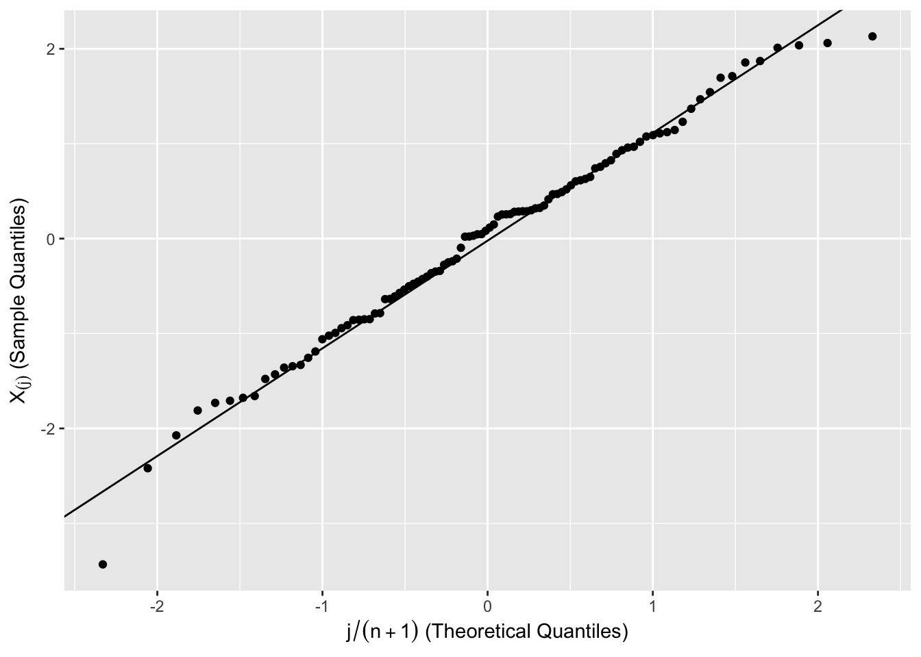
Figure 6.6: Normal Quantile Plot of 100 Simulated Observations from \(N(0,1)\)
These plots can be used to evaluate the normality of the effects in a \(2^k\) factorial design. Let \(\hat {\theta_{(1)}} < \hat {\theta_{(2)}} < \cdots < \hat {\theta_{(N)}}\) be \(N\) ordered factorial estimates. If we plot the points
\[(\hat {\theta_{i}} \thinspace, \thinspace \Phi^{-1}(p_i)), \thinspace i = 1,...,N,\]
where, \(p_i=i/(N+1)\), then factorial effects \(\hat {\theta_{i}}\) that are close to 0 will fall along a straight line. Therefore, points that fall off the straight line will be declared significant.
The rationale is as follows:
Assume that the estimated effects \(\hat {\theta_{i}}\) are \(N(\theta, \sigma^2)\) (estimated effects involve averaging of \(N\) observations, and the CLT (Section 2.6) ensures averages are nearly normal, even for \(N\) as small as 8).
If \(H_0: \theta_i = 0, \thinspace i = 1,...,N\) is true, then all the estimated effects will be zero.
The resulting normal probability plot of the estimated effects will be a straight line.
Therefore, the normal quantile plot is testing whether all of the estimated effects have the same distribution (i.e. same means).
When some of the effects are nonzero, the corresponding estimated effects will tend to be larger and fall off the straight line. For positive effects, the estimates fall above the line and negative effects fall below the line. Figure 6.7 shows a normal quantile plot of the factorial effects for Example 6.1, where the points are labeled as the main effects, A, B, C, and interactions A:B, B:C, A:C, A:B:C.
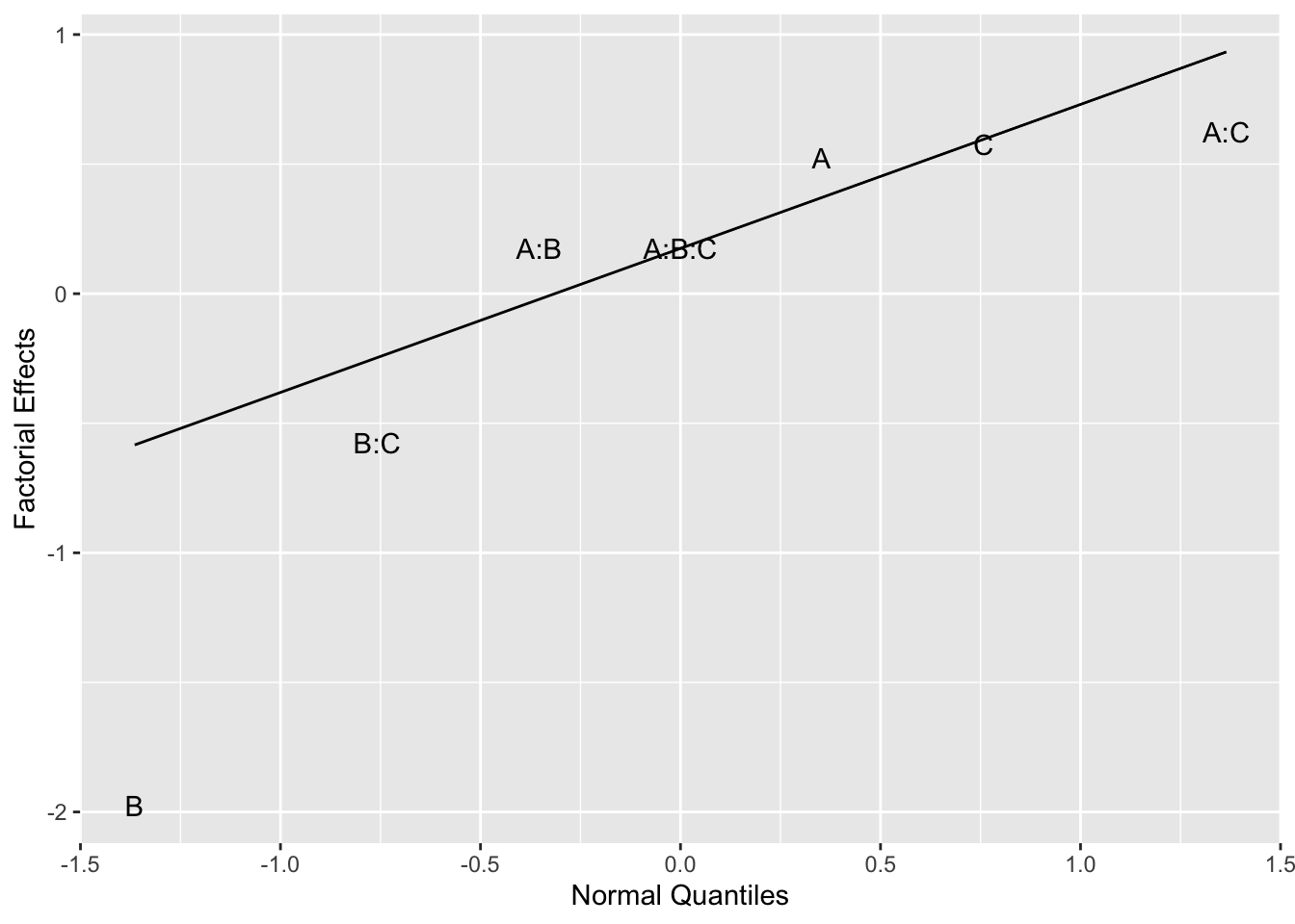
Figure 6.7: Normal Plot for Example 6.1
6.5.1 Half-Normal Plots
A related graphical method is called the half-normal probability plot. Let
\[\left|\hat{\theta}\right|_{(1)} < \left|\hat{\theta}\right|_{(2)} < \cdots < \left|\hat{\theta}\right|_{(N)}\]
be the ordered values of the absolute value of the factorial effect estimates. A normal quantile plot of the absolute value of factorial effects or half-normal plot can also be constructed.
Assume that the estimated effects \(\hat {\theta_{i}}\) are \(N(0, \sigma^2)\), so \(|\hat {\theta_{i}}|\) has p.d.f.
\[\frac{\sqrt{2}}{{\sigma}\sqrt{\pi}}\exp\left(-y^2/2\sigma^2\right),\thinspace y\ge 0. \] This is the p.d.f. of the half-normal distribution.
Suppose \(Y\) has a half-normal distribution with \(\sigma^2=1\). Let \(y_p\) be the \(p^{th}\) quantile of \(Y\), so \(p = F(y_p) = P(Y \le y_p)\). It can be shown that \(F(y_p) = 2(\Phi(y_p) -1/2))\). This implies that
\[y_p = F^{-1}(p) = \Phi^{-1}(p/2+1/2).\]
A quantile - quantile plot of the absolute values of factorial effects can use the standard normal CDF to compute the theoretical quantiles of the half-normal distribution.
The half-normal probability plot consists of the points
\[\left(\left|\hat{\theta}\right|_{(i)}, \Phi^{-1}(0.5+0.5[i-0.5]/N)\right), \thinspace i = 1,...,N.\]
This plot uses the first and third quantiles of the half-normal distribution to construct a comparative straight line.
An advantage of this plot is that all the large estimated effects appear in the upper right-hand corner and fall above the line. Figure 6.8 shows a half-normal plot of the factorial effects for Example 6.1. Normal plots can often be misleading. For example, Figure 6.7 suggests that the BC interaction might be interesting, even though it is smaller in magnitude than the AB effect. The half-normal plot avoids this visual trap. In this case, it shows that B is the only important effect.
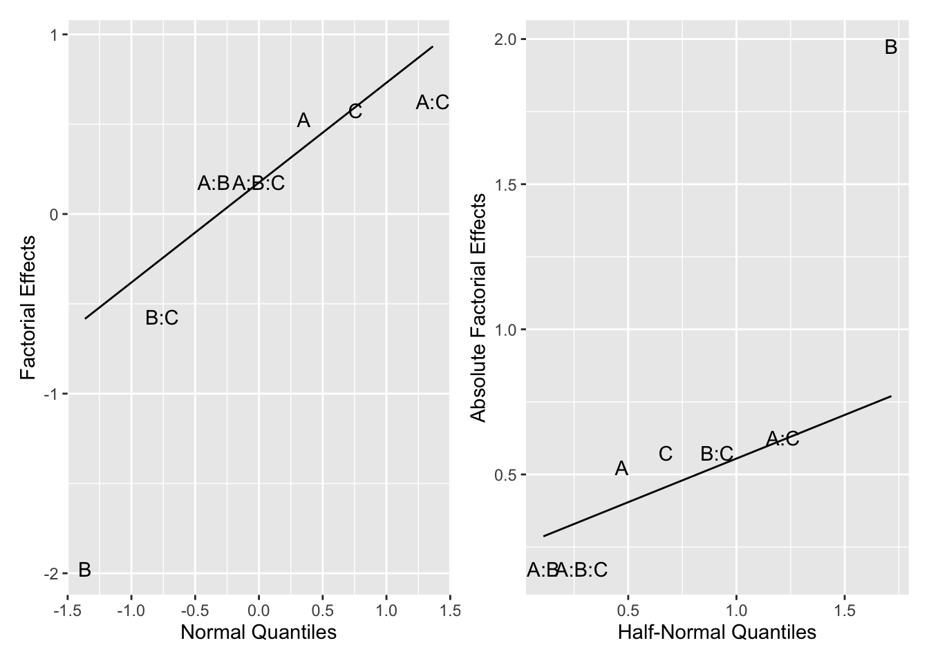
Figure 6.8: Full Normal and Half-Normal Plot for Example 6.1
6.5.2 Computation Lab: Normal Plots in Unreplicated Factorial Designs
Consider the data from the \(2^3\) design in Example 6.1. The factorial effects were estimated in Example 6.1 via a linear regression model in Section 6.4.1 and stored in fooddiary_mod. A vector of ordered factorial effects can be obtained using dplyr::arrange().
The normal quantile plot of factorial effects in Figure 6.7 was created using ggplot. To create the plot using the factor labels, we pass geom = "text" and label = rownames(effs) to ggplot2::geom_qq(). This tells ggplot2::geom_qq() to draw text using the rownames() of effs instead of the default geom = point. Finally, distribution = stats::qnorm specifies the distribution function to use.
ggplot(effs, aes(sample = theta)) +
  geom_qq(
    geom = "text",
    label = rownames(effs),
    distribution = stats::qnorm
  ) +
  geom_qq_line(distribution = stats::qnorm) +
  ylab("Factorial Effects") +
  xlab("Normal Quantiles")
A half-normal plot of the factorial effects can be created using ggplot() by computing the ordered absolute values of the factorial effects, and the corresponding theoretical quantiles of the half-normal and storing these values in a data frame.
effs <- data.frame(theta = abs(2 * coef(fooddiary_mod)[-1]))

effs <-
  effs %>%
  arrange(theta) %>%
  mutate(pi = qnorm(0.5 +
                      0.5 * (1:length(effs$theta) - 0.5) /
                      length(effs$theta)))
Instead of using ggplot2::geom_qq() and ggplot2::geom_qq_line(), geom_text() is used with label = rownames(effs) to draw the names of the factors.
ggplot(effs, aes(pi, theta)) +
  geom_text(label = rownames(effs)) +
  ylab("Absolute Factorial Effects") +
  xlab("half-Normal Quantiles")
Finally, a straight line is constructed that connects the first and third quartiles of the sample and theoretical quartiles. The quartile function of the half-normal distribution qhalf() is defined in terms of qnorm() and used to compute the intercept and slope of the straight line.
qhalf <- function(p) {
  qnorm(0.5 + 0.5 * p)
}

q <- quantile(effs$theta, c(0.25, 0.75))
slope <- (q[2] - q[1]) / (qhalf(.75) - qhalf(.25))
int <- q[1] - slope * qhalf(.25)
A reference line can be added to the plot using ggplot2::geom_abline().
ggplot(effs, aes(pi, theta)) +
  geom_text(label = rownames(effs)) +
  ylab("Absolute Factorial Effects") + xlab("half-Normal Quantiles") +
  geom_abline(intercept = int, slope = slope)
This code produces Figure 6.8.
BsMD::DanielPlot() creates normal and half-normal plots, although there is no option to add a reference line at this time.
6.6 Lenth’s Method
Half-normal and normal plots are informal graphical methods involving visual judgment. It’s desirable to judge a deviation from a straight line quantitatively based on a formal test of significance. Russell V Lenth51 proposed a method that is simple to compute and performs well.
Let
\[\hat{\theta}_{1},...,\hat{\theta}_{N} \]
be estimated factorial effects of \(\theta_1,\theta_2,...,\theta_N.\) Assume that all the factorial effects have the same standard deviation.
The pseudo standard error (PSE) is defined as
\[PSE = 1.5 \cdot \text{median}_{\left|\hat{\theta}_{i}\right|<2.5s_0}\left|\hat{\theta}_{i}\right|,\]
where the median is computed among the \(\left|\hat{\theta}_{i}\right|\) with \(\left|\hat{\theta}_{i}\right| < 2.5 s_0\) and
\[s_0 = 1.5 \cdot \text{median}\left|\hat{\theta}_{i}\right|.\]
\(1.5 \cdot s_0\) is a consistent estimator of the standard deviation of \(\hat \theta\) when \(\theta_i = 0\) and the underlying distribution is normal. The \(P\left(|Z|>2.57\right)=0.01\), \(Z\sim N(0,1)\). So, \(\left|\hat{\theta}_{i}\right|<2.5s_0\) trims approximately 1% of the \(\hat \theta_i\) if \(\theta_i = 0\). The trimming attempts to remove the \(\hat \theta_i\) associated with non-zero (active) effects. Using the median in combination with the trimming means that \(PSE\) is not sensitive to the \(\hat \theta_i\) associated with active effects.
To obtain a margin of error Lenth suggested multiplying the PSE by the \(100*(1-\alpha)\) quantile of the \(t_d\) distribution, \(t_{d,\alpha/2}\). The degrees of freedom is \(d = m/3\), where \(m\) is the number of factorial estimates.52 For example, the margin of error for a 95% confidence interval for \(\theta_i\) is
\[ME= t_{d,.025}\times PSE.\]
All estimates greater than the \(ME\) may be viewed as “significant,” but with so many estimates being considered simultaneously, some may be falsely identified.
A simultaneous margin of error that accounts for multiple testing can also be calculated,
\[SME = t_{d,\gamma} \times PSE,\]
where \(\gamma=\left(1+0.95^{1/N}\right)/2\).
6.6.1 Computation Lab: Lenth’s method
In this section, we will use Lenth’s method to test effect significance in the unreplicated \(2^3\) design presented in Example 6.1.
Let’s calculate Lenth’s method for the process development example. The estimated factorial effects are:
effs <- data.frame(theta = 2 * coef(fooddiary_mod)[-1])
round(effs, 2)
#>       theta
#> A      0.53
#> B     -1.97
#> C      0.58
#> A:B    0.17
#> A:C    0.62
#> B:C   -0.58
#> A:B:C  0.18
The estimate of \(s_0 = 1.5 \cdot \text{median}\left|\hat{\theta}_{i}\right|\) is
The trimming constant \(2.5s_0\) is
2.5 * s0
#> [1] 2.15625
The effects \(\hat{\theta}_{i}\) such that \({\left|\hat{\theta}_{i}\right| \ge 2.5s_0}\) will be trimmed. Below we mark the non-trimmed effects TRUE
cond <- abs(effs$theta) < 2.5 * s0
cond
#> [1] TRUE TRUE TRUE TRUE TRUE TRUE TRUE
The \(PSE\) is then calculated as 1.5 times the median of these values.
The \(ME\) and SME are
df_foodmod <- (2^3 - 1) / 3

ME <- PSE * qt(p = .975, df = df_foodmod)
ME
#> [1] 3.246556
SME <- PSE * qt(p = (1 + .95 ^ {
  1 / (8 - 1)
}) / 2, df = df_foodmod)
SME
#> [1] 7.769665
So, 95% confidence intervals, using the individual error rate, for the effects are
CI_L <- round(effs$theta - ME, 2)
CI_U <- round(effs$theta + ME, 2)
cbind(factor = rownames(effs),
      effects = round(effs$theta, 2),
      CI_L,
      CI_U)
#>      factor  effects CI_L    CI_U
#> [1,] "A"     "0.53"  "-2.72" "3.77"
#> [2,] "B"     "-1.97" "-5.22" "1.27"
#> [3,] "C"     "0.58"  "-2.67" "3.82"
#> [4,] "A:B"   "0.17"  "-3.07" "3.42"
#> [5,] "A:C"   "0.62"  "-2.62" "3.87"
#> [6,] "B:C"   "-0.58" "-3.82" "2.67"
#> [7,] "A:B:C" "0.18"  "-3.07" "3.42"
A plot of the effects with a \(ME\) and \(SME\) is usually called a Lenth plot. In R, it can be implemented via the function Lenthplot() in the BsMD library. The values of \(PSE\), \(ME\), and \(SME\) are part of the output. The spikes in the plot below are used to display factor effects.
BsMD::LenthPlot(fooddiary_mod)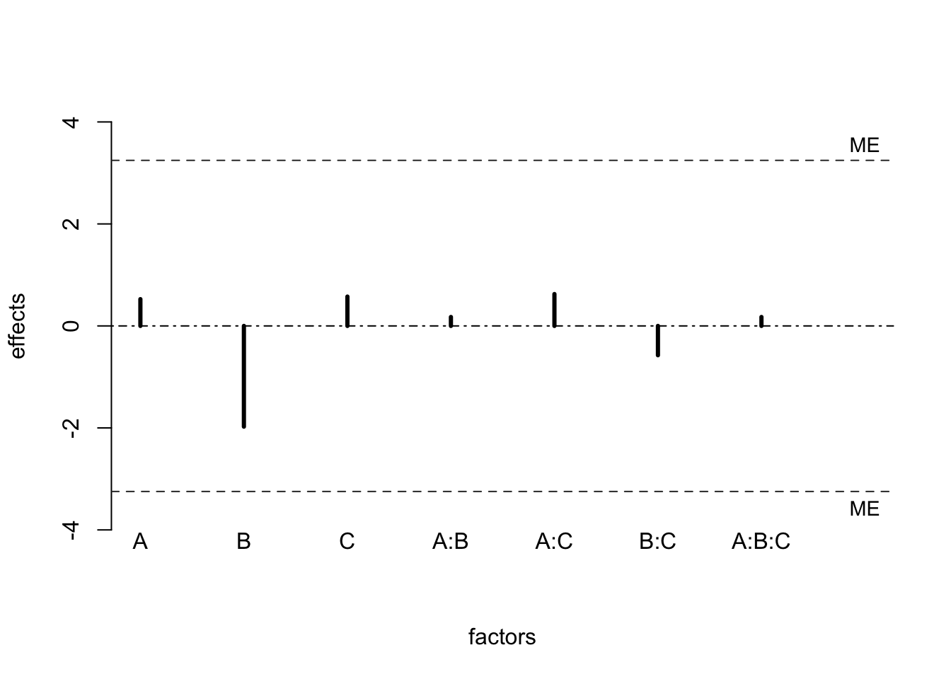
#>    alpha      PSE       ME      SME
#> 0.050000 0.862500 3.246556 7.769665
6.7 Blocking Factorial Designs
Blocking is usually used to balance the design with respect to a factor that may influence the outcome of interest and doesn’t interact with the experimental factors of interest. In the randomized block design discussed in Section 3.10, all treatments are compared in each block. This is feasible when the number of treatments doesn’t exceed the block size. In a \(2^k\) design, this is usually not realistic. One approach is to assign a fraction of the runs in a \(2^k\) design to each block.
Consider a \(2^3\) design that uses batches of raw material to create the treatment combinations, but the batches of raw material were only large enough to complete four runs of the experiment. Table 6.5 shows the design matrix for a \(2^3\) design in standard order, where the factors are labelled 1, 2, 3, and the interaction between factors 1 and 2 labelled as 12, etc. The levels of the variables are shown as \(-\) and \(+\) instead of \(+1\) and \(-1\).
| Run | 1 | 2 | 3 | 12 | 13 | 23 | 4=123 | Block |
|---|---|---|---|---|---|---|---|---|
| 1 | \(-\) | \(-\) | \(-\) | \(+\) | \(+\) | \(+\) | \(-\) | 1 |
| 2 | \(+\) | \(-\) | \(-\) | \(-\) | \(-\) | \(+\) | \(+\) | 2 |
| 3 | \(-\) | \(+\) | \(-\) | \(-\) | \(+\) | \(-\) | \(+\) | 2 |
| 4 | \(+\) | \(+\) | \(-\) | \(+\) | \(-\) | \(-\) | \(-\) | 1 |
| 5 | \(-\) | \(-\) | \(+\) | \(+\) | \(-\) | \(-\) | \(+\) | 2 |
| 6 | \(+\) | \(-\) | \(+\) | \(-\) | \(+\) | \(-\) | \(-\) | 1 |
| 7 | \(-\) | \(+\) | \(+\) | \(-\) | \(-\) | \(+\) | \(-\) | 1 |
| 8 | \(+\) | \(+\) | \(+\) | \(+\) | \(+\) | \(+\) | \(+\) | 2 |
Suppose that we assign runs 1, 4, 6, and 7 to block 1 which uses the first batch of raw material and runs 2, 3, 5, and 8 to block 2 which uses the second batch of raw material. The design is blocked this way by placing all runs in which the three-way interaction 123 is minus in one block and all the other runs in which 123 is plus in the other block (see Table 6.5).
Any systematic differences between the two blocks of four runs will be eliminated from all the main effects and two factor interactions. What you gain is the elimination of systematic differences between blocks. But now the three factor interaction is confounded with any batch (block) difference. The ability to estimate the three factor interaction separately from the block effect is lost.
6.7.1 Effect Heirarchy Principle
Lower-order effects are more likely to be important than higher-order effects.
Effects of the same order are equally likely to be important.
This principle suggests that when resources are scarce, priority should be given to the estimation of lower order effects. This is useful in screening experiments that have a large number of factors and a relatively small number of runs. Section 6.8 will discuss factorial designs that can study a large number of factors in a fraction of the runs needed in a full factorial design.
One reason that many accept this principle is that higher order interactions are more difficult to interpret or justify physically. As a result, investigators are less interested in estimating the magnitudes of these effects even when they are statistically significant.
Assigning a fraction of the \(2^k\) treatment combinations to each block results in an incomplete blocking (e.g., balanced incomplete block design). The factorial structure of a \(2^k\) design allows a neater assignment of treatment combinations to blocks. The neater assignment is done by dividing the total combinations into various fractions and finding optimal assignments by exploiting combinatorial relationships.
6.7.2 Generation of Orthogonal Blocks
In the \(2^3\) example in Table 6.5, the blocking variable is given the identifying number 4. Think of the study as containing four factors, where the fourth factor will have the special property that it does not interact with other factors. If this new factor is introduced by having its levels coincide exactly with the plus and minus signs attributed to 123, then the blocking is said to be generated by the relationship 4 = 123. This idea can be used to derive more sophisticated blocking arrangements.
Example 6.3 The following example is from Box, Hunter, and Hunter53. Consider an arrangement of a \(2^3\) design into four blocks using two block factors called 4 and 5 (see Table 6.6). 4 is associated with the three factor interaction, and 5 is associated with a the two factor interaction 23 which was deemed unimportant by the investigator. Runs are placed in different blocks depending on the signs of the block variables in columns 4 and 5. Runs for which the signs of 4 and 5 are \(--\) would go in one block, \(-+\) in a second block, \(+-\) in a third block, and \(++\) in the fourth.
| Block | Run |
|---|---|
| I | 4,6 |
| II | 3,5 |
| III | 1,7 |
| IV | 2,8 |
Block variables 4 and 5 are confounded with interactions 123 and 23. But there are three degrees of freedom associated with four blocks. The third degree of freedom accommodates the 45 interaction. But, the 45 interaction has the same signs as the main effect 1, since \(45=1\). Therefore, if we use 4 and 5 as blocking variables, then it will be confounded with block differences (see Table 6.6).
Main effects should not be confounded with block effects, and any blocking scheme that confounds main effects with blocks should not be used. This is based on the assumption that block-by-treatment interactions are negligible.
This assumption states that treatment effects do not vary from block to block. Without this assumption, estimability of the factorial effects will be very complicated.
For example, if \(B_1 = 12\) then this implies two other relations:
\[ 1B_1 = 1\times B_1 = 112 = 2 \thinspace {\text {and}} \thinspace B_12 = B_1 \times 2 = 122 = 1.\]
If there is a significant interaction between the block effect \(B_1\) and the main effect 1, then the main effect 2, is confounded with \(B_11\). Similarly, if there is a significant interaction between the block effect \(B_1\) and the main effect 2 then the main effect 1 is confounded with \(B_12\). Interactions can be checked by plotting the residuals for all the treatments within each block. If the pattern varies from block to block, then the assumption may be violated. A block-by-treatment interaction often suggests interesting information about the treatment and blocking variables.
| run | 1 | 2 | 3 | 12 | 13 | 5=23 | 4=123 | 45=1 |
|---|---|---|---|---|---|---|---|---|
| 1 | \(-\) | \(-\) | \(-\) | \(+\) | \(+\) | \(+\) | \(-\) | \(-\) |
| 2 | \(+\) | \(-\) | \(-\) | \(-\) | \(-\) | \(+\) | \(+\) | \(+\) |
| 3 | \(-\) | \(+\) | \(-\) | \(-\) | \(+\) | \(-\) | \(+\) | \(-\) |
| 4 | \(+\) | \(+\) | \(-\) | \(+\) | \(-\) | \(-\) | \(-\) | \(+\) |
| 5 | \(-\) | \(-\) | \(+\) | \(+\) | \(-\) | \(-\) | \(+\) | \(-\) |
| 6 | \(+\) | \(-\) | \(+\) | \(-\) | \(+\) | \(-\) | \(-\) | \(+\) |
| 7 | \(-\) | \(+\) | \(+\) | \(-\) | \(-\) | \(+\) | \(-\) | \(-\) |
| 8 | \(+\) | \(+\) | \(+\) | \(+\) | \(+\) | \(+\) | \(+\) | \(+\) |
6.7.3 Generators and Defining Relations
A simple calculus is available to show the consequences of any proposed blocking arrangement. If any column in a \(2^k\) design is multiplied by itself, a column of plus signs is obtained. This is denoted by the symbol \(I\). Thus, you can write
\[I = 11 = 22 = 33 = 44 = 55,\]
where, for example, 22 means the product of the elements of column 2 with itself.
Any column multiplied by \(I\) leaves the elements unchanged. So, \(I3 = 3\).
A general approach for arranging a \(2^k\) design in \(2^q\) blocks of size \(2^{k-q}\) is as follows. Let \(B_1, B_2, ...,B_q\) be the block variables, and the factorial effect \(v_i\) is confounded with \(B_i\),
\[B_1 = v_1,B_2 = v_2,...,B_q = v_q.\]
The block effects are obtained by multiplying the \(B_i\)’s:
\[B_1B_2 = v_1v_2, B_1B_3 = v_1v_3,...,B_1B_2 \cdots B_q = v_1v_2 \cdots v_q\]
There are \(2^{q}-1\) possible products of the \(B_i\)’s and the \(I\) (whose components are +).
Example 6.4 A \(2^5\) design can be arranged in eight blocks of size four.
Consider two blocking schemes.
Blocking scheme 1: Define the blocks as
\[B_1 = 135, B_2 = 235, B_3 = 1234.\] The remaining blocks are confounded with the following interactions:
\[B_1B_2 = 12, B_1B_3 = 245,B_2B_3 = 145,B_1B_2B_3 = 34\]
In this blocking scheme, the seven block effects are confounded with the seven interactions
\[12,34,135,145,235,245,1234.\]
Blocking scheme 2:
\[B_1 = 12, B_2 = 13, B_3 = 45.\]
This blocking scheme confounds the following interactions.
\[12, 13, 23,45, 1245,1345,2345.\]
Which is a better blocking scheme?
The second scheme confounds four two-factor interactions, while the first confounds only two two-factor interactions. Since two-factor interactions are more likely to be important than three- or four-factor interactions, the first scheme is superior.
6.7.4 Computation Lab: Blocking Factorial Designs
A \(2^3\) design in standard order can be generated by FrF2::FrF2(). nruns is the number of runs which is \(2^3=8\) in this case; the number of factors nfactors is 3, and randomize = FALSE (this tells FrF2() to keep runs in standard order; if randomize = TRUE then the order of the runs is randomized, i.e., not in standard order).
FrF2::FrF2(nruns = 8,
           nfactors = 3,
           randomize = FALSE)
#> creating full factorial with 8 runs ...
#>    A  B  C
#> 1 -1 -1 -1
#> 2  1 -1 -1
#> 3 -1  1 -1
#> 4  1  1 -1
#> 5 -1 -1  1
#> 6  1 -1  1
#> 7 -1  1  1
#> 8  1  1  1
#> class=design, type= full factorial
A \(2^k\) design generated by \(2^q\) blocks of size \(2^{k-q}\) can be generated using FrF2() using the blocks parameter. For example, a \(2^5\) design can be arranged in \(2^3\) blocks by defining blocks using the three independent variables \(\bf B_1=135, B_2=235,\) and \(\bf B_3=1234\). FrF2 factors are labelled with capital letters starting from the beginning of the alphabet.
This design is aliased or confounded with two two-factor interactions, and FrF2() will give an error message in this case. Specifying alias.block.2fis = TRUE will generate the design, and the aliasing information is available through aliased.with.blocks.
d325 <- FrF2::FrF2(
  nruns = 32,
  nfactors = 5,
  randomize = F,
  blocks = c("ACE", "BCE", "ABCD"),
  alias.block.2fis = TRUE
)
design.info(d325)$aliased.with.blocks
#> [1] "AB" "CD"
Consider an alternative blocking scheme, where \(\bf B_1=12, B_2=13,\) and \(\bf B_3=45\).
d325 <- FrF2::FrF2(
  nruns = 32,
  nfactors = 5,
  randomize = F,
  blocks = c("AB", "AC", "DE"),
  alias.block.2fis = TRUE
)
design.info(d325)$aliased.with.blocks
#> [1] "AB" "AC" "BC" "DE"
This blocking scheme is confounded with four two-factor interactions. Therefore, the first blocking scheme is preferred.
6.8 Fractional Factorial Designs
A \(2^k\) full factorial requires \(2^k\) runs. Full factorials are seldom used in practice for large k (k>=7). For economic reasons fractional factorial designs, which consist of a fraction of full factorial designs, are used. There are criteria to choose “optimal” fractions.
Consider a design that studies six factors in 32 (\(2^5\)) runs, which is a \(\frac{1}{2}\) fraction of a \(2^6\) factorial design. The design is referred to as a \(2^{6-1}\) design, where 6 denotes the number of factors and \(2^{-1}\) denotes the fraction. An important issue that arises in the design of these studies is how to select the fraction.
Example 6.5 (Treating HSV-1 with Drug Combinations) Jessica Jaynes et al.54 used a \(2^{6-1}\) fractional factorial design to a investigate a biological system with HSV-1 (Herpes simplex virus type 1) and six antiviral drugs. All combinations of six drugs, A, B, C, D, E, and F, were studied in 32 runs. The low and high levels of each drug were coded as \(-1\) and \(+1\). Table 6.7 displays the design matrix and data. The levels of drug F is the product of A, B, C, D, and E, that is, \(F = ABCDE\). The outcome variable, readout, is the percentage of cells positive for HSV-1 after combinatorial drug treatments.
| Run | A | B | C | D | E | F | Readout |
|---|---|---|---|---|---|---|---|
| 1 | -1 | -1 | -1 | -1 | -1 | -1 | 31.6 |
| 2 | -1 | -1 | -1 | -1 | 1 | 1 | 32.6 |
| 3 | -1 | -1 | -1 | 1 | -1 | 1 | 13.4 |
| 4 | -1 | -1 | -1 | 1 | 1 | -1 | 13.2 |
| 5 | -1 | -1 | 1 | -1 | -1 | 1 | 27.5 |
| 6 | -1 | -1 | 1 | -1 | 1 | -1 | 32.5 |
| 7 | -1 | -1 | 1 | 1 | -1 | -1 | 11.6 |
| 8 | -1 | -1 | 1 | 1 | 1 | 1 | 20.8 |
| 9 | -1 | 1 | -1 | -1 | -1 | 1 | 37.2 |
| 10 | -1 | 1 | -1 | -1 | 1 | -1 | 51.6 |
| 11 | -1 | 1 | -1 | 1 | -1 | -1 | 14.1 |
| 12 | -1 | 1 | -1 | 1 | 1 | 1 | 19.9 |
| 13 | -1 | 1 | 1 | -1 | -1 | -1 | 27.3 |
| 14 | -1 | 1 | 1 | -1 | 1 | 1 | 40.2 |
| 15 | -1 | 1 | 1 | 1 | -1 | 1 | 19.3 |
| 16 | -1 | 1 | 1 | 1 | 1 | -1 | 23.3 |
| 17 | 1 | -1 | -1 | -1 | -1 | 1 | 31.2 |
| 18 | 1 | -1 | -1 | -1 | 1 | -1 | 32.6 |
| 19 | 1 | -1 | -1 | 1 | -1 | -1 | 14.2 |
| 20 | 1 | -1 | -1 | 1 | 1 | 1 | 22.4 |
| 21 | 1 | -1 | 1 | -1 | -1 | -1 | 32.7 |
| 22 | 1 | -1 | 1 | -1 | 1 | 1 | 41.0 |
| 23 | 1 | -1 | 1 | 1 | -1 | 1 | 20.1 |
| 24 | 1 | -1 | 1 | 1 | 1 | -1 | 18.7 |
| 25 | 1 | 1 | -1 | -1 | -1 | -1 | 29.6 |
| 26 | 1 | 1 | -1 | -1 | 1 | 1 | 42.3 |
| 27 | 1 | 1 | -1 | 1 | -1 | 1 | 18.5 |
| 28 | 1 | 1 | -1 | 1 | 1 | -1 | 20.0 |
| 29 | 1 | 1 | 1 | -1 | -1 | 1 | 30.9 |
| 30 | 1 | 1 | 1 | -1 | 1 | -1 | 34.3 |
| 31 | 1 | 1 | 1 | 1 | -1 | -1 | 19.4 |
| 32 | 1 | 1 | 1 | 1 | 1 | 1 | 23.4 |
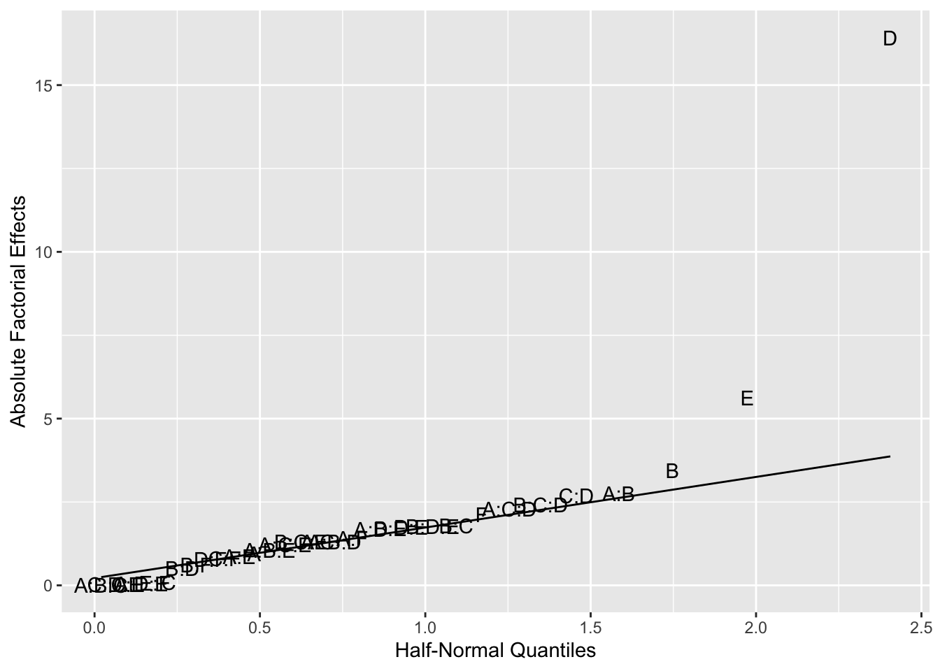
Figure 6.9: Half-Normal for Example 6.5
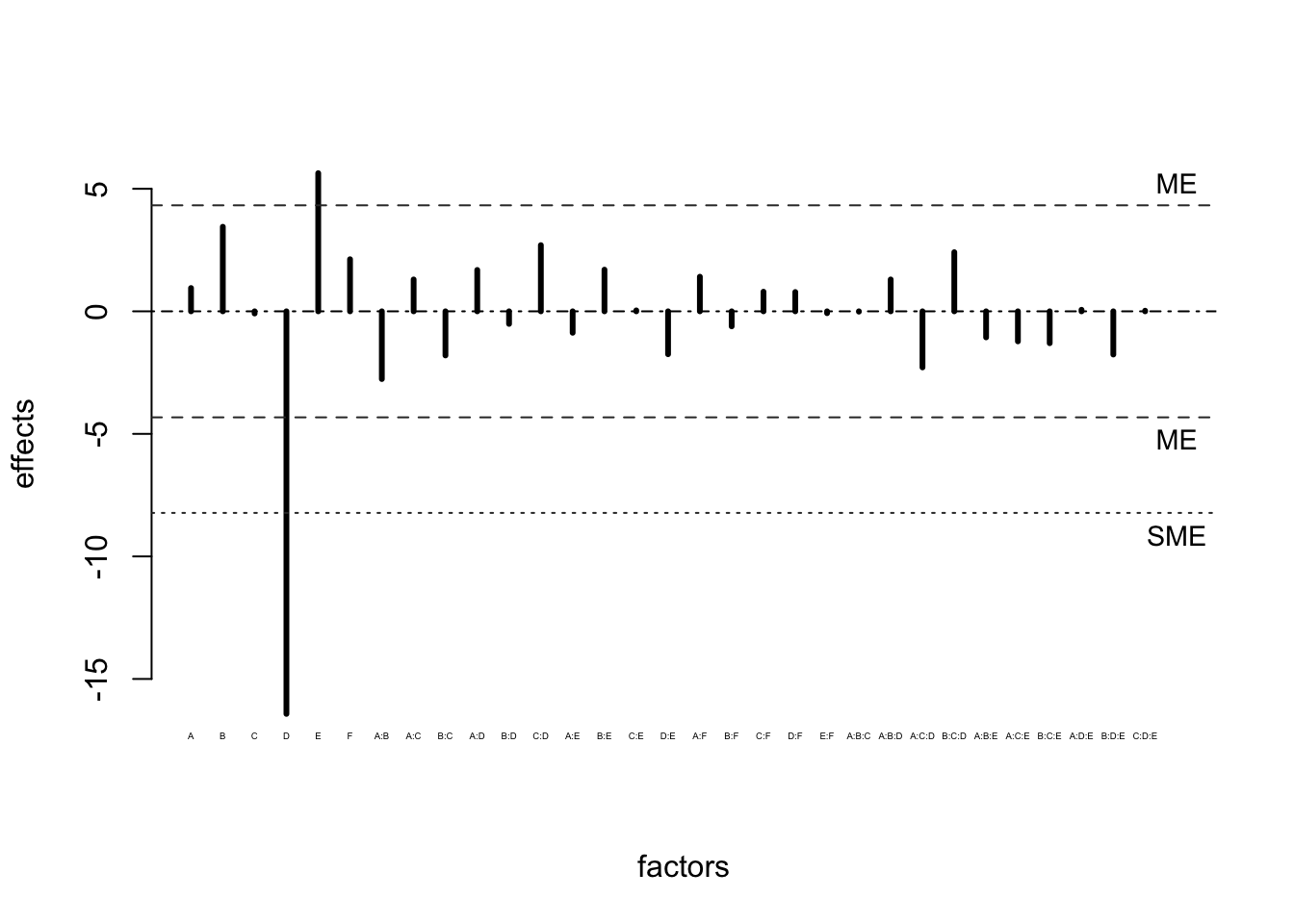
Figure 6.10: Lenth Plot for Example 6.5
6.8.1 Effect Aliasing and Design Resolution
Figures 6.9 and 6.10 both indicate that factors E and D may be effective in treating HSV-1. What information could have been obtained if a full \(2^6\) design had been used?
| Factors | Number of effects |
|---|---|
| Main | \({6 \choose 1} =\) 6 |
| 2-factor | \({6 \choose 2} =\) 15 |
| 3-factor | \({6 \choose 3} =\) 20 |
| 4-factor | \({6 \choose 4} =\) 15 |
| 5-factor | \({6 \choose 5} =\) 6 |
| 6-factor | \({6 \choose 6} =\) 1 |
There are 63 degrees of freedom in a 64 run design. But, 42 are used for estimating three factor interactions or higher. Is it practical to commit two-thirds the degrees of freedom to estimate such effects? According to the effect hierarchy principle, three-factor interactions and higher are not usually important. Thus, using full factorial is wasteful. It’s more economical to use a fraction of a full factorial design that allows lower order effects to be estimated.
The \(2^{6-1}\) design in Example 6.5 assigned the factor F to the five-way interaction ABCDE, so this design cannot distinguish between F and ABCDE. The main factor F is said to be aliased with the ABCDE interaction.
This aliasing relation is denoted by
\[F = ABCDE \thinspace \text{ or } \thinspace I = ABCDEF,\] where \(I\) denotes the column of all +’s.
This uses the same mathematical definition as the confounding of a block effect with a factorial effect. Aliasing of the effects is the price for choosing a smaller design.
The \(2^{6-1}\) design has only 31 degrees of freedom for estimating factorial effects, so cannot estimate all 63 factorial effects among the factors A, B, C, D, E, and F.
The equation \(I = ABCDEF\) is called the defining relation of the \(2^{6-1}\) design. The design is said to have resolution V because the defining relation consists of the “word” ABCDE, which has “length” 5.
Multiplying both sides of \(I = ABCDEF\) by column A
\[A = A \times I = A \times ABCDEF = BCDEF,\]
the relation \(A = BCDEF\) is obtained. A is aliased with the BCDEF interaction. The aliasing effect for the two-factor interaction AB is obtained by multiplying both sides of \(I=ABCDEF\) by \(AB\)
\[AB = AB \times I = AB \times ABCDEF=CDEF.\]
The two-factor interaction AB is aliased with the four-factor interaction CDEF. Table 6.8 shows all 31 aliasing relations for the design in Example 6.8.
| Alias |
|---|
| A = BCDEF |
| B = ACDEF |
| C = ABDEF |
| D = ABCEF |
| E = ABCDF |
| F = ABCDE |
| AB = CDEF |
| AC = BDEF |
| BC = ADEF |
| AD = BCEF |
| BD = ACEF |
| CD = ABEF |
| AE = BCDF |
| BE = ACDF |
| CE = ABDF |
| DE = ABCF |
| AF = BCDE |
| BF = ACDE |
| CF = ABDE |
| DF = ABCE |
| EF = ABCD |
| ABC = DEF |
| ABD = CEF |
| ACD = BEF |
| BCD = AEF |
| ABE = CDF |
| ACE = BDF |
| BCE = ADF |
| ADE = BCF |
| BDE = ACF |
| CDE = ABF |
6.8.2 Computation Lab: Fractional Factorial Designs
The design in Example 6.5 has six main effects with aliases: A = BCDEF, B = ACDEF, C = ABDEF, D = ABCEF, E = ABCDF, F = ABCDE. Therefore, the main effects of A, B, C, D, E, and F are estimable only if the aforementioned five-factor interactions are negligible. The other factorial effects have analogous aliasing properties.
The techniques that were covered for analysis of factorial designs are applicable to fractional factorial designs.
The FrF2() function can also be used for generating fractional factorial designs. The design for Example 6.5 is generated using FrF2::FrF2().
FrF2::FrF2(
  nruns = 32,
  nfactors = 6,
  factor.names = c("E", "D", "C", "B", "A", "F"),
  randomize = F
)
The data frame hsvdat contains the design matrix and dependent variable readout for Example 6.5. The factorial effects can be calculated using linear regression.
hsv_mod <- lm(readout ~ A * B * C * D * E * F, data = hsvdat)
2 * coef(hsv_mod)[-1]
#>           A           B           C           D           E
#>      0.9500      3.4500     -0.0875    -16.4250      5.6375
#>           F         A:B         A:C         B:C         A:D
#>      2.1250     -2.7625      1.3000     -1.8000      1.6875
#>         B:D         C:D         A:E         B:E         C:E
#>     -0.5125      2.7000     -0.8750      1.7000      0.0375
#>         D:E         A:F         B:F         C:F         D:F
#>     -1.7500      1.4125     -0.6125      0.8000      0.7875
#>         E:F       A:B:C       A:B:D       A:C:D       B:C:D
#>     -0.0750     -0.0125      1.3000     -2.2875      2.4125
#>       A:B:E       A:C:E       B:C:E       A:D:E       B:D:E
#>     -1.0625     -1.2250     -1.3000      0.0625     -1.7625
#>       C:D:E       A:B:F       A:C:F       B:C:F       A:D:F
#>      0.0250          NA          NA          NA          NA
#>       B:D:F       C:D:F       A:E:F       B:E:F       C:E:F
#>          NA          NA          NA          NA          NA
#>       D:E:F     A:B:C:D     A:B:C:E     A:B:D:E     A:C:D:E
#>          NA          NA          NA          NA          NA
#>     B:C:D:E     A:B:C:F     A:B:D:F     A:C:D:F     B:C:D:F
#>          NA          NA          NA          NA          NA
#>     A:B:E:F     A:C:E:F     B:C:E:F     A:D:E:F     B:D:E:F
#>          NA          NA          NA          NA          NA
#>     C:D:E:F   A:B:C:D:E   A:B:C:D:F   A:B:C:E:F   A:B:D:E:F
#>          NA          NA          NA          NA          NA
#>   A:C:D:E:F   B:C:D:E:F A:B:C:D:E:F
#>          NA          NA          NA
The aliases can be computed using the FrF2::aliases().
FrF2::aliases(hsv_mod)
#>
#>  A = B:C:D:E:F
#>  B = A:C:D:E:F
#>  C = A:B:D:E:F
#>  D = A:B:C:E:F
#>  E = A:B:C:D:F
#>  F = A:B:C:D:E
#>  A:B = C:D:E:F
#>  A:C = B:D:E:F
#>  B:C = A:D:E:F
#>  A:D = B:C:E:F
#>  B:D = A:C:E:F
#>  C:D = A:B:E:F
#>  A:E = B:C:D:F
#>  B:E = A:C:D:F
#>  C:E = A:B:D:F
#>  D:E = A:B:C:F
#>  A:F = B:C:D:E
#>  B:F = A:C:D:E
#>  C:F = A:B:D:E
#>  D:F = A:B:C:E
#>  E:F = A:B:C:D
#>  A:B:C = D:E:F
#>  A:B:D = C:E:F
#>  A:C:D = B:E:F
#>  B:C:D = A:E:F
#>  A:B:E = C:D:F
#>  A:C:E = B:D:F
#>  B:C:E = A:D:F
#>  A:D:E = B:C:F
#>  B:D:E = A:C:F
#>  C:D:E = A:B:F
6.9 Exercises
Exercise 6.1 Consider a \(4^2 \times 3^2 \times 2\) factorial design.
How many factors are included in this design?
How many levels are included in each factor?
How many experimental conditions, or runs, are included in this design?
Exercise 6.2 Consider a \(2^2\) factorial experiment with factors A and B. Show that \(INT(A,B)=INT(B,A)\). That is, the interaction is symmetric in B and A.
Exercise 6.3 Consider a \(2^3\) experiment with factors A, B, and C. Show that
\[\begin{split} INT(A,B,C) =& \frac{1}{2}\left[ INT\left(\left.A,C\right|B+\right) - INT\left(\left.A,C\right|B-\right) \right] \\ =& \frac{1}{2}\left[ INT\left(\left.C,B\right|A+\right) - INT\left(\left.C,B\right|A-\right) \right]. \end{split}\]
Exercise 6.4 Example 6.1 used
sum(wtlossdat["B"]*wtlossdat["y"])/4to compute the main effect of C.
Explain why the espression is divided by 4?
Write an R function to calculate the main effects using the design matrix.
Write an R function to calculate the interaction effects using the design matrix.
Exercise 6.5 Show that the variance of the \(i^{th}\) run in a \(2^3\) design with two replications is
\[\frac{\left(y_{i1}-y_{i2}\right)^2}{2},\]
where \(y_{ij}\) is \(j^{th}\) observation in \(i^{th}\) experimental run.
Exercise 6.6 Show that the variance of a factorial effect in a \(2^k\) design with \(m\) replications is
\[\frac{4\sigma^2}{N},\]
where \(N = m\cdot 2^k\) and \(\sigma^2\) is the variance of each outcome.
Exercise 5.1 Assume that \(y_{ij}\) are i.i.d and follow a normal distribution with variance \(\sigma^2\). Under the null hypothesis that a factorial effect 0,
- Show that
\[\frac{\bar y_+ - \bar y_-}{s\left/2\right.}\sim t_{2^k(m - 1)}\]
in a \(2^k\) design with \(m\) replications.
- Suppose that \(y_{ij}\) are not normal. Why is it still reasonable to assume that the ratio of the factorial effect to its standard error follows a normal distribution?
Exercise 6.7 Use R to calculate the three-way interaction effects from the experiment in Example 6.2. Interpret these interaction terms.
Exercise 6.8 This exercise is based on Section 5.2 of Box, Hunter, and Hunter55. An experiment for optimizing response yield (y) in a chemical plant operation was conducted. The three factors considered are temperature (T), concentration (C), and catalyst type (K). The order of the runs (run) was randomized. The levels for the factors are listed below.
| Factor | Level |
|---|---|
| T. Temperature (\(^{\circ}\)C) 1 | 60 (-1), 180(+1) |
| C. Concentration (%) | 20 (-1), 40 (+1) |
| K. Catalyst | A (-1), B (+1) |
The data are available in the chemplant data frame.
glimpse(chemplant, n = 3)
#> Rows: 16
#> Columns: 5
#> $ run <int> 6, 2, 1, 5, 8, 9, 3, 7, 13, 4, 16, 10, 12, 14,…
#> $ T   <int> -1, 1, -1, 1, -1, 1, -1, 1, -1, 1, -1, 1, -1, …
#> $ C   <int> -1, -1, 1, 1, -1, -1, 1, 1, -1, -1, 1, 1, -1, …
#> $ K   <int> -1, -1, -1, -1, 1, 1, 1, 1, -1, -1, -1, -1, 1,…
#> $ y   <int> 59, 74, 50, 69, 50, 81, 46, 79, 61, 70, 58, 67…
State the design.
Use R to calculate all the factorial effects.
Which factors have an important effect on yield? Explain how you arrived at your answer.
Exercise 5.3 Interpret the intercept term in the linear regression model represented in Example 6.1.
Exercise 5.4 Suppose that a \(2^2\) factorial design studying factors A and B was conducted. An investigator fits the model
\[y_i = \beta_0 x_{i0}+\beta_1 x_{i1} + \beta_2 x_{i2} + \beta_3 x_{i3} + \epsilon_i,\]
\(i,\dots,n\), to estimate the factorial effects of the study.
What is the value of \(n\)? Define \(x_{ik}, k = 0, 1, 2, 3\).
Derive the least-squares estimates of \(\beta_k, k = 0, 1, 2,3.\)
Show that the least-squares estimates of A, B, AB, are one-half the factorial effects.
Exercise 6.9 Suppose that linear regression is used to estimate factorial effects for a \(2^k\) design by doubling the estimated regression coefficients.
When is it possible to estimate the standard error of these regression coefficients?
If the p-values for the regression coefficients are able to be calculated, then is it necessary to transform these p-values to correspond to p-values for factorial effects? Explain.
Exercise 5.5 Suppose \(Y\) has a half-normal distribution with variance \(\sigma^2=1\). Let \(y_p\) be the \(p^{th}\) quantile of \(Y\) such that \(p = F(y_p)\) and \(\Phi\) be the CDF of the standard normal distribution.
Show that \(F(y_p) = 2\Phi(y_p)-1\).
Show that the \(p^{th}\) quantile of a half-normal is \(y_p= \Phi^{-1}\left(p\left/2\right. + 1\left/2\right.\right)\).
Exercise 2.12 In Section 6.5.2 Computation Lab: Normal Plots in Unreplicated Factorial Designs, the factorial effects were sorted based on their magnitudes before plotting the normal quantile plot shown in Figure 6.7.
Create the normal quantile plot without sorting the factorial effects. What is wrong with the plot?
Instead of using
geom_qq()andgeom_qq_line(), construct a normal quantile plot usinggeom_point()and add an appropriate straight line to the plot that connects the first and third quantiles of the theoretical and sample distributions.Suppose the absolute values of factorial effects are used in a normal quantile plot. Will the result be an interpretable plot to assess the significance of factorial effects in an unreplicated design? Explain.
Exercise 5.6 Reconstruct the half-normal plot shown in Figure 6.8 using geom_qq() and geom_qq_line().
Exercise 6.10 The planning matrix from a \(2^{k-p}\) design is below. The four factors investigated are A, B, C, and D.
| A | B | C | D |
|---|---|---|---|
| \(-\) | \(-\) | \(-\) | \(-\) |
| \(+\) | \(-\) | \(-\) | \(+\) |
| \(-\) | \(+\) | \(-\) | \(+\) |
| \(+\) | \(+\) | \(-\) | \(-\) |
What are the values of \(k\) and \(p\)?
What is the defining relation? What is the resolution of this design?
What are the aliasing relations?
Use
FrF2::FrF2()to generate this design.
Exercise 6.11 Use the FrF2()::FrF2() function to generate the design matrix in the standard order for a \(2^3\) design with blocks generated using the three-way interaction.
Exercise 6.12 An investigator is considering two blocking schemes for a \(2^4\) design with 4 blocks. The two schemes are listed below.
- Scheme 1: \(B_1=134\), \(B_2=234\)
- Scheme 2: \(B_1=12\), \(B_2=13\), \(B_3 = 1234\)
Which runs are assigned to which blocks in each scheme?
For each scheme, list all interactions confounded with block effects.
Which blocking scheme is preferred? Explain why.
Exercise 5.13 This exercise is based on Section 5.1 of CF Jeff Wu and Michael S Hamada56. An experiment to improve a heat treatment process on truck leaf springs was conducted. The heat treatment that forms the camber in leaf springs consists of heating in a high temperature furnace, processing by forming a machine, and quenching in an oil bath. The free height of an unloaded spring has a target value of 8 in. The goal of the experiment is to make the variation about the target as small as possible.
The five factors studied in this experiment are shown below. The data are available in the data frame leafspring, where y1, y2, y3 are three replications of the free height measurements.
| Factor | Level |
|---|---|
| B. Temperature | 1840 (-), 1880 (+) |
| C. Heating time | 23 (-), 25 (+) |
| D. Transfer time | 10 (-), 12 (+) |
| E. Hold down time | 2 (-), 3 (+) |
| Q. Quench oil temperature | 130-150 (-), 150-170 (+) |
glimpse(leafspring, n = 3)
#> Rows: 16
#> Columns: 8
#> $ B  <chr> "-", "+", "-", "+", "-", "+", "-", "+", "-", "+…
#> $ C  <chr> "+", "+", "-", "-", "+", "+", "-", "-", "+", "+…
#> $ D  <chr> "+", "+", "+", "+", "-", "-", "-", "-", "+", "+…
#> $ E  <chr> "-", "+", "+", "-", "+", "-", "-", "+", "-", "+…
#> $ Q  <chr> "-", "-", "-", "-", "-", "-", "-", "-", "+", "+…
#> $ y1 <dbl> 7.78, 8.15, 7.50, 7.59, 7.94, 7.69, 7.56, 7.56,…
#> $ y2 <dbl> 7.78, 8.18, 7.56, 7.56, 8.00, 8.09, 7.62, 7.81,…
#> $ y3 <dbl> 7.81, 7.88, 7.50, 7.75, 7.88, 8.06, 7.44, 7.69,…
Answer the questions below.
State the design.
What is the defining relation? Which of the factorial effects are aliased?
The goal of this experiment was to investigate which factors minimize variation of free height. Use the sample variance for each run as the dependent variable to estimate the factorial effects.
Which factorial effects have an important effect on free height variation?
Exercise 5.15 A baker (who is also a scientist) designs an experiment to study the effects of different amounts of butter, sugar, and baking powder on the taste of his chocolate chip cookies.
| Factor | Amount |
|---|---|
| B. Butter | 10g (-), 15g (+) |
| S. Sugar | 1/2 cup (-), 3/4 cup (+) |
| P. Baking Powder | 1/2 teaspoon (-), 1 teaspoon (+) |
The response variable is taste measured on a scale of 1 (poor) to 10 (excellent). He first designs a full factorial experiment based on the three factors butter, sugar, and baking powder. But, before running the experiment the baker decides to add another factor of baking time (T)—12 minutes vs. 16 minutes. However, he cannot afford to conduct more than 8 runs since each run requires time to prepare a different batch of cookie dough, bake the cookies, and measure taste. So, he decides to use the three factor interaction between butter, sugar, and baking powder to assign whether baking time will be 12 minutes (-) or 16 minutes (+) in each of the 8 runs.
The data frame cookies contains the data for this experiment, but does not contain a column for baking time.
glimpse(cookies)
#> Rows: 8
#> Columns: 5
#> $ Run    <dbl> 1, 2, 3, 4, 5, 6, 7, 8
#> $ Butter <dbl> -1, 1, -1, 1, -1, 1, -1, 1
#> $ Sugar  <dbl> -1, -1, 1, 1, -1, -1, 1, 1
#> $ Powder <dbl> -1, -1, -1, -1, 1, 1, 1, 1
#> $ Taste  <dbl> 3, 3, 10, 2, 6, 5, 4, 6
Add a column for baking time (T) to
cookies.State the design.
Which factors have an important effect on taste?
Are any of the factors aliased? If yes, then state the defining relation and aliasing effects.
The cookie batches were baked without randomizing the order of the runs. What impact, if any, would this have on the results? Explain.
In order to speed up the experiment, the baker was contemplating using his neighbour’s oven to bake runs 1, 4, 6, and 7. What impact, if any, could this have on the results? Explain.