5 Comparing More Than Two Treatments

5.1 Introduction: ANOVA—Comparing More Than Two Groups

Chapter 3 discussed design and analysis of comparing two treatments by randomizing experimental units to two different treatment groups. This chapter discusses design and analysis for comparing more than two treatments.

Example 5.1 (Three-arm randomized clinical trial) Adam W Amundson et al.³⁷ conducted a clinical trial of three different treatments to control pain during knee surgery. The primary outcome of the study was maximal pain (0 to 10, numerical pain rating scale where higher values indicate more severe pain) one day after surgery. The study aimed to enrol 150 participants randomized in equal numbers to the three treatments (in clinical trials, treatments are often called arms—short for treatment arms).

Table 5.1: Example 5.1 Treatment Means and Standard Deviations

trt	N	Mean	SD
A	50	6.20	1.34
B	50	7.32	1.15
C	50	3.64	1.51

Is there evidence to indicate a difference in mean pain scores for the three different pain treatments? An idea due to R.A. Fisher is to compare the variation in mean pain scores between the treatments to the variation of pain scores within a treatment. These two measures of variation are often summarized in an analysis of variance (ANOVA) table.

5.2 Random Assignment of Treatments

The number of possible randomizations in Example 5.1 is

\[{150 \choose{50 \thinspace 50 \thinspace 50}}= \frac{150!}{50!50!50!} \approx 2.03 \times 10^{69}.\]

One of the random allocations could be selected by taking a random permutation of the numbers 1 through 150 and then assigning the first 50 to the first treatment, the second 50 to the second treatment, etc. One of the drawbacks of this method is that the sample size in each group will be unequal until all the participants are randomized. In studies such as clinical trials, it’s common to plan an interim analysis before all the participants are enrolled to evaluate safety and efficacy. If the groups are unbalanced, then this could lead to a loss of power (see Chapter 4).

Permuted block randomization avoids this problem by randomizing experimental units within a smaller block of experimental units. The order of treatment assignments within a block are random, but the desired proportion of treatments is achieved in each block. In Example 5.1 participants could be randomized to treatments in a block size of 6: 2 assigned to treatment 1; 2 assigned to treatment 2; and 2 assigned to treatment 3. If the treatments are labeled A, B, and C then possible blocks could be: ABBACC, CABBCA, or CBAACB. As the blocks are filled, the study is guaranteed to have the desired allocation to each group.

5.2.1 Computation Lab: Random Assignment

A randomization scheme can be created for Example 5.1 by labeling participants with the sequence 1:150, selecting a random permutation, then assigning the first 50 to treatment A, etc.

set.seed(1)
subj <- sample(1:150)
trt <- c(rep("A", 50), rep("B", 50), rep("C", 50))
randscheme <- data.frame(subj, trt) %>% arrange(subj, trt)
head(randscheme)
#>   subj trt
#> 1    1   B
#> 2    2   A
#> 3    3   C
#> 4    4   C
#> 5    5   C
#> 6    6   A

Participant 1 is randomized to treatment B, etc. The treatment assignments to the first 6 participants indicate an unequal number of treatments since there are 2 A’s, 3 C’s, and 1 B.

A permuted block randomization will correct this issue. Consider blocks of size 6. To obtain a random order of treatments in block sizes of 6, we can replicate trts twice and then sample() the resulting vector to obtain a random permutation. The function create_blocks() creates blocks of size m \(\times\) length(trts).

trts <- c("A", "B", "C")

create_block <- function(m) {
  sample(rep(trts, m))
}

To create a randomization scheme with a block size of 6 for the study, we can run create_block() \(150/6=25\) times using replicate().

randscheme <- replicate(25, create_block(m = 2))

5.3 ANOVA

5.3.1 Source of Variation and Sums of Squares

Let \(y_{ij}, i=1,\ldots,k;j=1,\ldots n_i\) be the \(j^{th}\) observation with treatment \(i\). The \(i^{th}\) treatment mean will be denoted as \({\bar y}_{i\cdot}=y_{i\cdot}/{n_i}\), where \(y_{i\cdot}=\sum_{j = 1}^{n_i} y_{ij}.\) The grand (overall) mean is \({\bar y}_{\cdot \cdot}=y_{\cdot \cdot}/N\), where \(y_{\cdot \cdot}=\sum_{i = 1}^k \sum_{j = 1}^{n_i} y_{ij}.\) \(N = \sum_{i=1}^k n_i\) is the total number of observations. The “dot” subscript notation means sum over the subscript that it replaces.

Consider a scenario such as Example 5.1. The between treatments variation and within treatment variation are two components of the total variation in the response. We can break up each observation’s deviation from the grand mean \(y_{ij}-{\bar y}_{\cdot \cdot}\) into two components: treatment deviations \(\left(\bar y_{i \cdot}-{\bar y}_{\cdot \cdot}\right)\) and residuals within treatment deviations \(\left(y_{ij}-{\bar y}_{i \cdot}\right)\).

\[y_{ij}-{\bar y}_{\cdot \cdot}=\left(\bar y_{i \cdot}-{\bar y}_{\cdot \cdot}\right)+\left(y_{ij}-{\bar y}_{i \cdot}\right),\]

where \(y_{ij}\) is the \(jth\) observation, \(j=1,\ldots,n_i\) taken under treatment \(i = 1,...,k\).

The statistical model that we will study in this section is

\[\begin{equation} y_{ij}=\mu+\tau_i+\epsilon_{ij}, \tag{5.1} \end{equation}\]

where \(\tau_i\) is the \(ith\) treatment effect, and \(\epsilon_{ij} \sim N(0,\sigma^2)\) is the random error of the \(j^{th}\) observation in the \(i^{th}\) treatment. For example, the average of the observations under treatment one \((i=1)\), \(E\left(y_{1j}\right)\), minus the grand average, \(\mu\), \(\tau_1=E\left(y_{1j}\right)-\mu\) is the first treatment effect.

We are interested in testing whether the \(k\) treatment effects are equal.

\[H_0: \tau_1=\cdots=\tau_k \hspace{0.5cm}\text{vs.}\hspace{0.5cm} H_1: \tau_l \ne \tau_m, \thinspace l \ne m.\]

5.3.2 ANOVA Identity

The total sum of squares \(SS_{T}= \sum_{i = 1}^k \sum_{j = 1}^{n_i} \left(y_{ij}- {\bar y}_{\cdot \cdot}\right)^2\) can be written as

\[\sum_{i = 1}^k \sum_{j = 1}^{n_i} \left[({\bar y}_{i\cdot} - {\bar y}_{\cdot \cdot}) + (y_{ij}- {\bar y}_{i \cdot})\right]^2\]

by adding and subtracting \({\bar y}_{i\cdot}\) to \((y_{ij}- {\bar y}_{\cdot \cdot})\).

Expanding and summing the expression leads to

\[\begin{align} SS_T = \sum_{i = 1}^k \sum_{j = 1}^{n_i} \left(y_{ij}-{\bar y}_{\cdot \cdot}\right)^2 &= \underbrace{\sum_{i = 1}^k n_i\left(\bar{y_{i \cdot}}-{\bar y}_{\cdot \cdot}\right)^2}_{\text{Sum of Squares Due to Treatment}} + \underbrace{\sum_{i = 1}^k \sum_{j = 1}^{n_i} \left(y_{ij}-{\bar y}_{i \cdot} \right)^2}_{\text{Sum of Squares Due to Error}} \label{eq1} \\ &= SS_{Treat} + SS_E. \tag{5.2} \end{align}\]

This is sometimes called the analysis of variance identity. It shows how the total sum of squares can be split into two sums of squares: one part that is due to differences between treatments, and one part due to differences within treatments. The squared deviations \(SS_{Treat}\) are called the sum of squares due to treatments (i.e., between treatments), and \(SS_E\) is called the sum of squares due to error (i.e., within treatments).

5.3.3 Computation Lab: ANOVA Identity

R functions to compute \(SS_T\), \(SS_{Treat}\), and \(SS_E\) are below. SST() computes the sum of squared deviations: SSTreat() first splits the data frame into treatment groups then computes the sum of squared deviations of the treatment means sst multiplied by n the number of observations within a treatment group, and finally SSe() computes the sum of squared deviations of each observation within a treatment from its treatment mean. lapply() is used in SSTreat() and SSe() to compute the function over a vector or list and returns a list, unlist() converts the list to a vector so that we can apply sum().

SST <- function(y) {
  sum((y - mean(y)) ^ 2)
}

SSTreat <- function(y, groups, n) {
  sst <- unlist(lapply(split(y, groups),
                       function(x) {
                         (mean(x) - mean(y)) ^ 2
                       }))
  return(n * sum(sst))
}

SSe <- function(y, groups) {
  sum(unlist(lapply(split(y, groups),
                    function(x) {
                      (x - mean(x)) ^ 2
                    })))
}

The painstudy data frame contains data for Example 5.1, and the ANOVA identity (5.2) can be verified using the functions above.

5.3.4 ANOVA: Degrees of Freedom

Suppose you are asked to choose a pair of real numbers \((x,y)\) at random. This means that you have complete freedom to choose the two numbers, or two degrees of freedom. Now, suppose that you are asked to choose a pair of real numbers \((x,y)\), such that \(x+y=10\). Once you choose, say \(x\), then \(y\) is fixed, so there is only one degree of freedom in this case.

What are the degrees of freedom of \(SS_T\)? There are \(N=\sum_{i}^kn_i\) residual terms \((y_{ij}-\bar y_{\cdot \cdot})\), such that \(\sum_{i=1}^k \sum_{j=1}^{n_i}(y_{ij}-\bar y_{\cdot \cdot})=0\). This means that any \(N-1\) are completely determined by the other. Therefore, \(SS_T\) has \(N-1\) degrees of freedom. Similarly, \(SS_{Treat}\) has \(k-1\) degrees of freedom. Within each treatment there are \(n_i\) observations with \(n_i-1\) degrees of freedom, and there are \(k\) treatments. So, there are \(\sum_{i=1}^k(n_i-1) = N-k\) degrees of freedom for \(SS_E\).

5.3.5 ANOVA: Mean Squares

\[SS_E= \sum_{i = 1}^k \left[\sum_{j = 1}^{n_i} \left(y_{ij}-{\bar y}_{i \cdot} \right)^2\right]\]

If the term inside the brackets is divided by \(n-1\), then it is the sample variance for the \(ith\) treatment

\[S_i^2=\frac{\sum_{j = 1}^{n_i} \left(y_{ij}-{\bar y}_{i \cdot} \right)^2}{(n_i-1)}, \hspace{1cm} 1 = 1,...,k.\]

Combining these \(k\) variances to give a single estimate of the common population variance,

\[\frac{(n_1-1)S_1^2+ \cdots + (n_k-1)S_k^2}{(n_1-1)+ \cdots + (n_k-1)}=\frac{SS_E}{N-k}.\]

It can be shown that \(E(SS_E)=(N-k)\sigma^2.\) So, \(SS_E/(N-k)\) can be used to estimate \(\sigma^2\).

If there were no differences between the \(k\) treatment means \({\bar y}_{i \cdot}\) we could use the variation of the treatment averages from the grand average to estimate \(\sigma^2\).

\[\frac{SS_{Treat}}{k-1}.\]

It can be shown that \(E(SS_{Treat})=k\sum_{i=1}^k \tau_i^2+(k-1)\sigma^2.\) So, if \(\tau_i=0\), then \(SS_{Treat}/(k-1)\) is an estimate of \(\sigma^2\) when the treatment deviations are all equal.

The analysis of variance identity can be used to give two estimates of \(\sigma^2\): one based on the variability within treatments and the other based on the variability between treatments. These two estimators of \(\sigma^2\) are called mean square treatment and error.

Definition 5.1 (Mean Square for Treatment) The mean square for treatment is defined as \[MS_{Treat}=\frac{SS_{Treat}}{k-1}.\]

Definition 5.2 (Mean Square for Error) The mean square for error is defined as

\[MS_E=\frac{SS_E}{N-k}.\]

5.3.6 ANOVA: F Statistic

It can be shown that \(SS_{Treat}\) and \(SS_E\) are independent. If \(H_0: \tau_1=\cdots=\tau_k=0\) is true, then then \(SS_{Treat}/\sigma^2 \sim \chi^2_{k-1}\) and \(SS_E/\sigma^2 \sim \chi^2_{N-k}\), so

\[ F= \frac{MS_{Treat}}{MS_E} \sim F_{k-1,N-k}.\]

5.3.7 ANOVA Table

A table that records the source of variation, degrees of freedom, sum of squares, mean squares, and F statistic values is called an ANOVA table.

Table 5.2: ANOVA Table

Source of variation	Degrees of freedom	Sum of squares	Mean square	F
Between treatments	\(k-1\)	\(SS_{Treat}\)	\(MS_{Treat}\)	\(F\)
Within treatments	\(N-k\)	\(SS_E\)	\(MS_E\)

Where, \(F=\frac{MS_{Treat}}{MS_E}\).

5.3.8 Computation Lab: ANOVA Table

The aov() function fits an ANOVA model and the summary() function computes the ANOVA table. The ANOVA table for Example 5.1 is

anova_mod <- aov(pain ~ trt, data = painstudy)
summary(anova_mod)
#>              Df Sum Sq Mean Sq F value Pr(>F)    
#> trt           2  355.8   177.9   98.92 <2e-16 ***
#> Residuals   147  264.4     1.8                   
#> ---
#> Signif. codes:  
#> 0 '***' 0.001 '**' 0.01 '*' 0.05 '.' 0.1 ' ' 1

5.4 Estimating Treatment Effects Using Least Squares

The statistical model for ANOVA (5.1) can also be described as a linear regression model (2.4).

5.4.1 Dummy Coding

In Example 5.1, \(y_{ij}\) is the \(j^{th}\) pain score, \(j=1,\ldots,50\) for the \(i^{th}\) treatment group, \(i=1,2,3\), which correspond to treatments A, B, and C, respectively.

Table 5.3: First Six Observations of Example 5.1

A	B	C
6	8	3
7	5	1

Let \({\bf y} = \underbrace{(y_{11},y_{21}, \ldots, y_{50 \thinspace 3})^{\prime}}_{150 \times 1}\) represent the column vector \((6,8,3, \ldots,5,9,6)^{\prime}\),

\[X=\begin{pmatrix} 1 & x_{11} & x_{12} \\ 1 & x_{21} & x_{22} \\ \vdots & \vdots & \vdots \\ 1 & x_{150 \thinspace 1} & x_{150 \thinspace2} \end{pmatrix} ,\quad {\boldsymbol \beta}= \begin{pmatrix} \mu \\ \tau_1 \\ \tau_2 \end{pmatrix}, \quad {\boldsymbol \epsilon}=\begin{pmatrix} \epsilon_{11} \\ \epsilon_{21} \\ \vdots \\ \epsilon_{3\thinspace50} \end{pmatrix}\]

where,

\[x_{1j} = \left\{ \begin{array}{ll} 1 & \mbox{if jth unit receives treatment B } \\ 0 & \mbox{otherwise} \end{array} \right.,\]

\[x_{2j} = \left\{ \begin{array}{ll} 1 & \mbox{if jth unit receives treatment C } \\ 0 & \mbox{otherwise} \end{array} \right..\]

This regression model implicitly assumes that the regression parameter for treatment A is zero (e.g., \(\tau_3=0\)). This is often called the baseline constraint.

The predictors \(x_{1j}\) and \(x_{2j}\) are coded as dummy variables; dummy coding compares each level to a reference level, and the intercept is the mean of the reference group. In this example, we have used two categorical covariates, coded as dummy variables, to describe three treatments (see Section 2.8.3); otherwise the regression model would be overparameterized and \((X^{\prime}X)^{-1}\) would not exist.

We can also write the regression model using (2.3)

\[\begin{equation} y_{ij}=\mu+\tau_1x_{1j}+\tau_2x_{2j}+\epsilon_{ij}. \tag{5.3} \end{equation}\]

If \(i=3\), then \(E(y_{3j})=\mu\), the intercept of this model, is the mean pain score of the treatment A group. Letting \(\mu=\mu_A\) and using a similar notation for the other treatments:

\[\begin{aligned} E(y_{1j})=\mu_B=\mu+\tau_1 &\Rightarrow \tau_1=\mu_B-\mu_A, \\ E(y_{2j})=\mu_C=\mu+\tau_2 &\Rightarrow \tau_2=\mu_C-\mu_A. \end{aligned}\]

Using (2.5) we can obtain the least squares estimates:

\[\begin{aligned} {\hat \mu}={\bar y}_{1 \cdot}, \quad {\hat \tau_1}={\bar y}_{2 \cdot}-{\bar y}_{1 \cdot}, \quad {\hat \tau_2}&={\bar y}_{3 \cdot }-{\bar y}_{1 \cdot}. \end{aligned}\]

5.4.2 Deviation Coding

This coding system compares the mean of the dependent variable for a given level to the overall mean of the dependent variable. Suppose the independent variables in model (5.3) are defined as

\[x_{1j} = \left\{ \begin{array}{ll} 1 & \mbox{if treatment A } \\ -1 & \mbox{if treatment C} \\ 0 & \mbox{otherwise} \end{array} \right., \quad x_{2j} = \left\{ \begin{array}{ll} 1 & \mbox{if treatment B} \\ -1 & \mbox{if treatment C} \\ 0 & \mbox{otherwise} \end{array} \right.\]

This coding is equivalent to assuming a regression model where \(\tau_1+\tau_2+\tau_3=0\), where \(\tau_3\) is the regression parameter for treatment C. This is often called the zero-sum constraint. It is another type of constraint on the regression model to ensure that \(X^{\prime}X\) is non-singular.

1 is used to compare a level to all other levels and -1 is assigned to treatment C because it’s the level that will never be compared to the other levels.

Let \(i=1\), so \(\mu_A=E(y_{1j})\). Then \(\mu_A=\mu + \tau_1\) is the mean pain score of the treatment A group. Continuing with this notation, we have \(\mu_B=\mu+\tau_2\), and \(\mu_C=\mu-\tau_1-\tau_2\). Solving for \(\mu\), \(\tau_1\), and \(\tau_2\), we have

\[\begin{aligned} \mu = \frac{\mu_A+\mu_B+\mu_C}{3}, \quad \tau_1 = \mu_A-\mu, \quad \tau_2 = \mu_B-\mu. \end{aligned}\]

5.5 Computation Lab: Estimating Treatment Effects Using Least Squares

lm() can be used to fit a linear regression model that calculates estimates of the ANOVA treatment effects. In this section, we will use the data in Example 5.1. The dependent variable is pain and the independent variable is trt. But, let’s start with checking the coding of trt using stats::contrasts().

painstudy$trt is a character vector, but contrasts() takes a factor vector as an argument. So, we can use as.factor() to convert to an R factor object.

painstudy$trt <- as.factor(painstudy$trt)
contrasts(painstudy$trt)
#>   B C
#> A 0 0
#> B 1 0
#> C 0 1

The output shows a matrix whose columns define dummy variables \(x_{1j}\) and \(x_{2j}\) with treatment A as the reference category (since it has a row of 0’s). This coding (i.e., contrast) is the default in R for unordered factors, and can be specified using contr.treatment(). To change the reference category, use the base option in contr.treatment().

contrasts(painstudy$trt) <- contr.treatment(n = 3, base = 2)
contrasts(painstudy$trt)
#>   1 3
#> A 1 0
#> B 0 0
#> C 0 1

contr.treatment(n = 3, base = 2) indicates that there are n = 3 treatment levels, and the reference category is the second category base = 2 (the default is base = 1). Contrast can also be specified in lm().

aovregmod <- lm(pain ~ trt,
                data = painstudy,
                contrasts = 
                  list(trt = contr.treatment(n = 3, base = 2)))
broom::tidy(aovregmod)
#> # A tibble: 3 × 5
#>   term        estimate std.error statistic  p.value
#>   <chr>          <dbl>     <dbl>     <dbl>    <dbl>
#> 1 (Intercept)     7.32     0.190     38.6  8.17e-79
#> 2 trt1           -1.12     0.268     -4.18 5.07e- 5
#> 3 trt3           -3.68     0.268    -13.7  4.22e-28

Table 5.1 gives the treatment means. The estimate of treatment B mean is the (Intercept) term (7.32); the estimate for trt1 is the difference between the means for treatments A (6.2) and B (7.32); and the estimate for trt3 corresponds to the difference between the means for treatments C (3.64) and B (7.32).

confint(aovregmod)
#>                 2.5 %     97.5 %
#> (Intercept)  6.945178  7.6948222
#> trt1        -1.650079 -0.5899214
#> trt3        -4.210079 -3.1499214

Confidence intervals for the treatment estimates can be obtained using the confint() function. Neither confidence interval for the treatment effects contain zero so would be considered statistically significant at the 5% level (this can also be ascertained by examining the p-values in summary(aovregmod)).

Alternatively, we could use deviation coding by specifying the contrast as contr.sum().

contrasts(painstudy$trt) <- contr.sum(3)
contrasts(painstudy$trt)
#>   [,1] [,2]
#> A    1    0
#> B    0    1
#> C   -1   -1

In this contrast, treatment C is never compared to the other treatments. If we wish to change this to, say, treatment A, then use the levels argument of factor() to reorder the levels of a factor.

painstudy$trt <- factor(painstudy$trt, levels = c("C", "B", "A"))
contrasts(painstudy$trt) <- contr.sum(3)
contrasts(painstudy$trt)
#>   [,1] [,2]
#> C    1    0
#> B    0    1
#> A   -1   -1

Now, we can fit the regression model with deviation coding where treatment A is the comparison treatment.

aovregmod <- lm(pain ~ trt, data = painstudy)
broom::tidy(aovregmod)
#> # A tibble: 3 × 5
#>   term        estimate std.error statistic  p.value
#>   <chr>          <dbl>     <dbl>     <dbl>    <dbl>
#> 1 (Intercept)     5.72     0.110      52.2 8.13e-97
#> 2 trt1           -2.08     0.155     -13.4 2.42e-27
#> 3 trt2            1.60     0.155      10.3 3.77e-19

The (Intercept) is the grand mean or mean of means \((\) 6.2 + 7.32 + 3.64 \()/3=\) 5.72; trt1 is the mean of treatment C 3.64 minus the the grand mean, and trt2 is the mean of treatment B 7.32 minus the grand mean.

5.5.1 ANOVA Assumptions

The calculations that make up an ANOVA table require no assumptions. You could complete the table using the ANOVA identity and definitions of mean square and F statistic for a data set with \(k\) treatments. However, using these numbers to make inferences about differences in treatment means requires certain statistical assumptions.

1. Additive model. The observations \(y_{ij}\) can be modelled as the sum of treatment effects and random error, \(y_{ij}=\mu+\tau_i+\epsilon_{ij}.\) The parameters \(\tau_i\) are interpreted is the \(i^{th}\) treatment effect.

2. Under the assumption that the errors \(\epsilon_{ij}\) are independent and identically distributed with a common variance \(Var(\epsilon_{ij})=\sigma^2\), for all \(i,j\), \(E(MS_{Treat})=(k/k-1)\sum_{i = 1}^k \tau_i^2 + \sigma^2, \mbox{and } E(MS_E)=\sigma^2.\) If \(\tau_i=0, i=1,\ldots,k\) then \(E(MS_{treat})=E(MS_E)=\sigma^2\).

3. If \(\epsilon_{ij} \sim N(0,\sigma^2)\) then \(MS_{Treat}\) and \(MS_E\) are independent. Under the null hypothesis, \(H_0:\tau_i=0, i=1,\ldots,a\), the ratio \(F={MS_{Treat}}/{MS_E} \sim F_{a-1,N-a}\).

5.5.2 Computation Lab: Checking ANOVA Assumptions

In this section, we check the ANOVA assumptions (Section 5.5.1) for Example 5.1.

1. The ANOVA decomposition implies acceptance of the additive model \(y_{ij}=\mu+\tau_j+\epsilon_{ij},\) where \(\mu\) is the mean of treatment A and \(\tau_j\) is the deviation produced by treatment \(j\), and \(\epsilon_{ij}\) is the associated random error. There are no formal methods that we have introduced to check this assumption.

2. The common variance assumption can be investigated by plotting the residuals versus the fitted values of the ANOVA model. A plot of the residuals versus fitted values can be used to investigate the assumption that the residuals are randomly distributed and have constant variance. Ideally, the points should randomly fall on both sides of 0, with no recognizable patterns in the points. In R, this can be done using the following commands.

data.frame(resid = aovregmod$residuals, 
           pred = aovregmod$fitted.values) %>%
  ggplot(aes(x = pred, y = resid)) +
  geom_point() +
  geom_hline(yintercept = 0)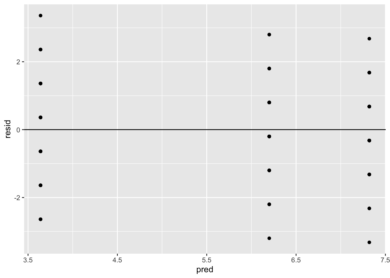

The assumption of constant variance is satisfied since there is no recognizable pattern.

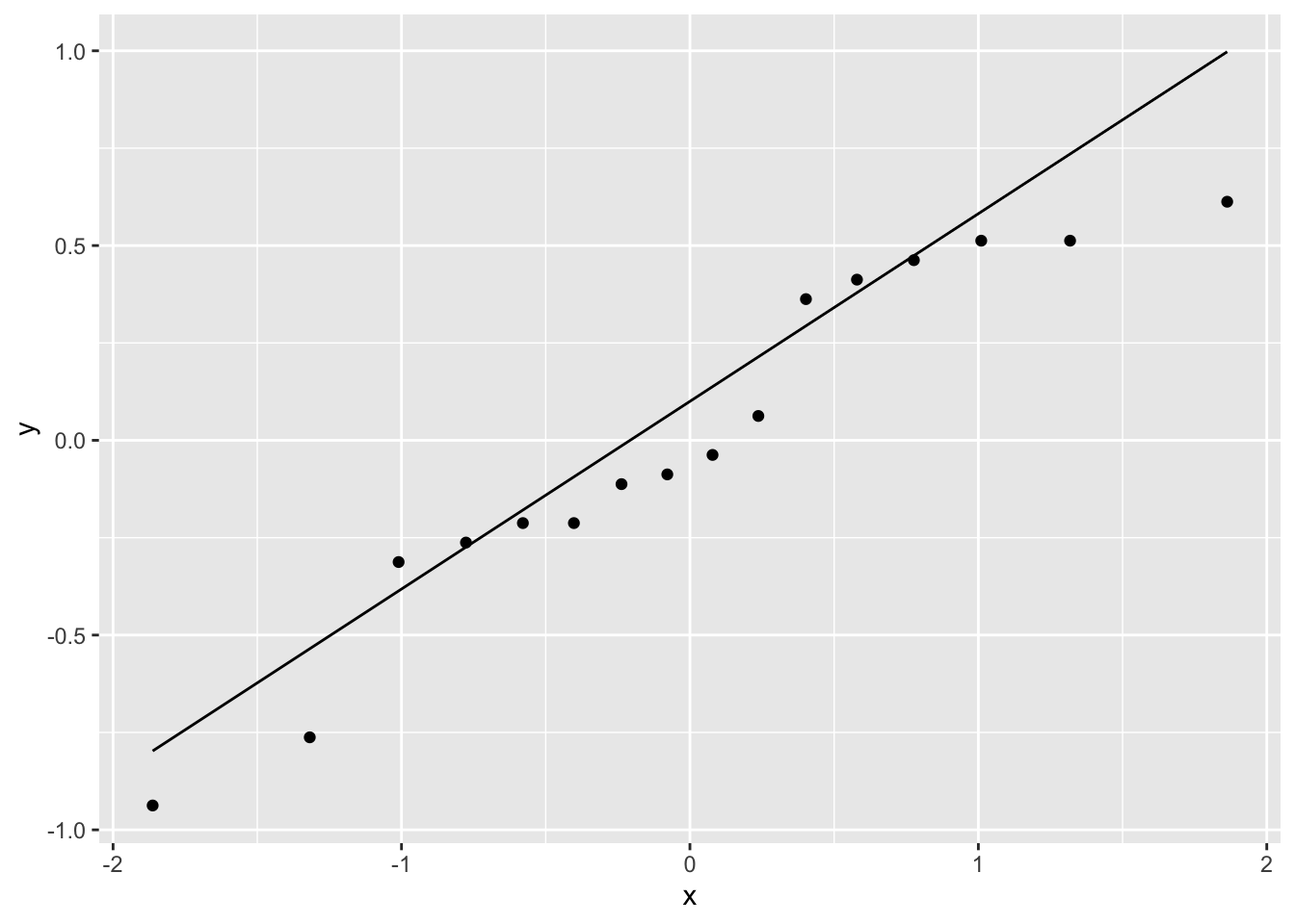
3. The normality of the residuals can be investigated using a normal quantile-quantile plot (see 2.5).

5.6 Multiple Comparisons

Suppose that experimental units were randomly assigned to three treatment groups. The hypothesis of interest is

\[H_0: \mu_1=\mu_2 =\mu_3 \thinspace {\text vs. } \thinspace H_1: \mu_i \ne\mu_j.\]

If \(H_0\) is rejected at level \(\alpha\), then which pairs of means are significantly different from each other at level \(\alpha\)? There are \({3 \choose 2}=3\) possibilities.

1. \(\mu_1 \ne \mu_2\)
2. \(\mu_1 \ne \mu_3\)
3. \(\mu_2 \ne \mu_3\)

Suppose that \(k = 3\) separate (independent) hypothesis level \(\alpha\) tests are conducted:

\[H_{0_k}: \mu_i=\mu_j \thinspace {\text vs. } \thinspace H_{1_k}: \mu_i \ne\mu_j.\]

When \(H_0\) is true, \(P_{H_0}\left(\text{reject } H_0 \right)=\alpha \Rightarrow P_{H_0}\left(\text{not reject } H_0 \right)=1-\alpha\). So, if \(H_0\) is true, then

\[\begin{aligned} P_{H_0}\left(\text{reject at least one } H_{0_k} \right) &= 1- P_{H_0}\left(\text{not reject any } H_{0_k} \right) \\ &= 1- P_{H_0}\left(\text{not reject } H_{0_1} \text{and } \text{not reject } H_{0_2} \text{and } \text{not reject } H_{0_3} \right) \\ &= 1- P_{H_0}\left(\text{not reject } H_{0_1}\right)P\left(\text{not reject } H_{0_2}\right)P\left(\text{not reject } H_{0_3}\right) \hspace{0.3cm} \\ &= 1-(1-\alpha)^{3} \end{aligned}\]

If \(\alpha = 0.05\) then the probability that at least one \(H_0\) will be falsely rejected is \(1-(1-.05)^3 = 0.14\), which is almost three times the type I error rate.

In general if \[H_0: \mu_1=\mu_2 = \cdots =\mu_k \thinspace {\text vs. } \thinspace H_1: \mu_i \ne\mu_j,\]

and \(c={k \choose 2}\) independent hypotheses are conducted, then the probability

\[P_{H_0}\left(\text{reject at least one } H_{0_k} \right) = 1-(1-\alpha)^c\]

is called the family-wise error rate (FWER).

The pairwise error rate is \(P_{H_0}\left(\text{reject } H_{0_k} \right)=\alpha\) for any \(c\).

The multiple comparisons problem is that multiple hypotheses are tested at level \(\alpha\) which increases the probability that at least one of the hypotheses will be falsely rejected (family-wise error rate).

When an ANOVA F test is significant, then investigators often wish to explore where the differences lie. Is it appropriate to test for differences looking at all pairwise comparisons when testing all possible pairs increases the type I error rate? An increased type I error rate (e.g. 0.14) means that that there is a higher probability of detecting a significant difference when no difference exists.

In the next two sections, we will cover two methods, Bonferroni and Tukey, for adjusting the p-values so that the FWER does not increase when all pairwise comparisons are conducted.

5.6.1 The Bonferroni Method

To test for the difference between the \(ith\) and \(jth\) treatments, it is common to use the two-sample t-test. The two-sample \(t\) statistic is

\[ t_{ij}= \frac{\bar{y_{j \cdot}}-\bar{y_{i \cdot}} } {\hat{\sigma}\sqrt{1/n_j+1/n_i}},\]

where \(\bar{y_{j \cdot}}\) is the average of the \(n_i\) observations for treatment \(j\) and \(\hat{\sigma}\) is \(\sqrt{MS_E}\) from the ANOVA table.

Treatments \(i\) and \(j\) are declared significantly different at level \(\alpha\) if

\[|t_{ij}|>t_{N-k,1-\alpha/2}.\]

The total number of pairs of treatment means that can be tested is

\[c={k \choose 2}=\frac{k(k-1)}{2}.\]

The Bonferroni method for testing \(H_0:\mu_i=\mu_j\) vs. \(H_0:\mu_i \ne \mu_j\) rejects \(H_0\) at level \(\alpha\) if

\[|t_{ij}|>t_{N-k,\alpha/2c},\]

where \(c\) denotes the number of pairs being tested.

5.6.2 The Tukey Method

Treatments \(i\) and \(j\) are declared significantly different at level \(\alpha\) if

\[|t_{ij}|>\frac{1}{\sqrt 2} q_{k,N-k,\alpha},\]

where \(t_{ij}\) is the observed value of the two-sample t-statistic and \(q_{k,N-k,\alpha}\) is the upper \(\alpha\) percentile of the Studentized range distribution with parameters \(k\) and \(N-k\) degrees of freedom.

A 100\((1-\alpha)\)% simultaneous confidence interval for \(c\) pairs \(\mu_i-\mu_j\) is

\[\bar{y_{j \cdot}}-\bar{y_{i \cdot}} \pm \frac{1}{\sqrt 2} q_{k,N-k,\alpha} \hat{\sigma}\sqrt{1/n_j+1/n_i}.\]

The Bonferroni method is more conservative than Tukey’s method. In other words, the simultaneous confidence intervals based on the Tukey method are shorter.

The main difference between the Tukey and Bonferroni methods is in the choice of the critical value.

5.6.3 Computation Lab: Multiple Comparisons

Example 5.2 (Four-arm randomized clinical trial) A pain study similar to Example 5.1 was conducted, except that 120 participants were randomized to four pain treatments during knee surgery in equal numbers. The primary outcome of the study was maximal pain (0 to 10, numerical pain rating scale where higher values indicate more severe pain) one day after surgery. The goal of the study was to evaluate which treatments were effective. The data for this study is in the data frame painstudy2.

The library emmeans³⁸ has functions that can compute estimated treatment (also called marginal) means, comparisons and contrasts with adjusted p-values and confidence intervals. emmeans() computes the marginal means, and pairs() computes all pairwise comparisons with an option to adjust the comparisons using tukey or bonferroni.

We first fit a regression model and then compute the means for each trt using emmeans::emmeans().

library(emmeans)
painstudy2mod <- lm(pain ~ trt, data = painstudy2)
painstud.emm <- emmeans(painstudy2mod, specs = "trt")
painstud.emm
#>  trt emmean    SE  df lower.CL upper.CL
#>  A     6.60 0.237 116     6.13     7.07
#>  B     7.37 0.237 116     6.90     7.84
#>  C     3.20 0.237 116     2.73     3.67
#>  D     7.20 0.237 116     6.73     7.67
#> 
#> Confidence level used: 0.95

To obtain all \({4 \choose 2}=6\) pairwise comparisons with the Tukey adjustment we use the pairs() function with adjust = tukey, and using confint() adds confidence intervals for each comparison.

ci <- confint(pairs(painstud.emm, adjust = "tukey"))

Unadjusted 95% confidence intervals are obtained using adjust = "none".

confint(pairs(painstud.emm, adjust = "none"))
#>  contrast estimate    SE  df lower.CL upper.CL
#>  A - B      -0.767 0.335 116   -1.431  -0.1023
#>  A - C       3.400 0.335 116    2.736   4.0644
#>  A - D      -0.600 0.335 116   -1.264   0.0644
#>  B - C       4.167 0.335 116    3.502   4.8310
#>  B - D       0.167 0.335 116   -0.498   0.8310
#>  C - D      -4.000 0.335 116   -4.664  -3.3356
#> 
#> Confidence level used: 0.95

Adjusting for multiple comparisons in this case has an impact on statistical signifcance at the 5% level, since the comparison A - B is no longer significant after the Tukey adjustment. Alternatively, the CDF and inverse CDF of the Studentized Range Distribution stats::ptukey() and stats::qtukey() could be used directly to compute the confidence intervals.

We can also obtain plots of the adjusted confidence intervals.

plot(painstud.emm, comparisons = TRUE, adjust = "tukey")
pwpp(painstud.emm, comparisons = TRUE, adjust = "tukey")

An explanation on how to interpret these plots is given by Lenth³⁹.

5.7 Sample Size for ANOVA—Designing a Study to Compare More Than Two Treatments

When designing a study to compare more than two treatments, investigators often need to consider how many experimental units will be assigned to each group to detect differences if they exist. In this section the methods introduced in Chapter 4 are extended to ANOVA.

\[\begin{equation} H_0: \mu_1=\mu_2 = \cdots = \mu_k \thinspace {\text vs. } \thinspace H_1: \mu_i \ne\mu_j. \tag{5.4} \end{equation}\]

is an ANOVA test comparing \(k\) treatment means. The test rejects at level \(\alpha\) if

\[MS_{Treat}/MS_E \ge F_{k-1,N-K,\alpha}.\]

The power of the test is \(P_{H_1}\left(MS_{Treat}/MS_E \ge F_{k-1,N-K,\alpha} \right)\). In order to compute this probability, we require the distribution of \(MS_{Treat}/MS_E\) when \(H_0\) is false. It can be shown that \(MS_{Treat}/MS_E\) has a non-central \(F\) distribution with the numerator and denominator degrees of freedom \(k-1\) and \(N-k\) respectively, and non-centrality parameter

\[\begin{equation} \delta = \frac{\sum_{i = 1}^kn_i\left(\mu_i-{\bar \mu} \right)^2}{\sigma^2}, \tag{5.5} \end{equation}\]

where \(n_i\) is the number of observations in group \(i\), \({\bar \mu}=\sum_{i = 1}^k \mu_i/k\), and \(\sigma^2\) is the within group error variance.

Let \(F_{a,b}(\delta)\) denote the non-central \(F\) distribution with numerator and denominator degrees of freedom \(a,b\) and non-centrality parameter \(\delta\).

The power of (5.4) is \(P\left(F_{k-1,N-k}(\delta) > F_{k-1,N-K,\alpha} \right),\) where \(\delta\) is defined in (5.5).

A few important properties of this power function include:

• The power is an increasing function in \(\delta\)
• The power depends on the true values of the treatment means \(\mu_i\), the within group error variance \(\sigma^2\), and sample size \(n_i\).
• The degrees of freedom used in the power function are \(k-1\) for the numerator degrees of freedom (\(k\) is the number of groups) and \(N-k\) for the denominator degrees of freedom, where \(N = \sum_{i=1}^k n_i\) (\(n_i\) is the total number of observations in group \(i\)) is the total number of observations.

An investigator could also design a study by specifying an effect size. In this case, the effect size is the standard deviation of the population means divided by the common within-population standard deviation.

\[f = \sqrt{\frac{\sum_{i = 1}^k\left(\mu_i-{\bar \mu} \right)^2/k}{\sigma^2}}.\]

\({\bar \mu}=\sum_{i = 1}^k \mu_i/k\), and \(\sigma^2\) is the within group error variance.

When the number of experimental units per group is constant, the relationship between effect size \(f\) for ANOVA and the non-centrality parameter \(\delta\) is

\[\begin{equation} \delta = knf^2, \tag{5.6} \end{equation}\]

where \(n_i=n\) is the number of observations in group \(i = 1,...,k\).

5.7.1 Computation Lab: Sample Size for ANOVA

5.7.1.1 Power Function

Power of the ANOVA test can be computed directly by writing a function to compute (5.5) and then using the R functions qf() and pf() for the \(F\) quantile and distribution functions.

anovancp <- function(n, mu, sigma) {
  mubar <- mean(mu)
  sum(n * (mu - mubar) ^ 2) / sigma ^ 2
}

Suppose that an investigator hypothesizes that the true means are \(\mu_1=1\), \(\mu_2=1.5\), \(\mu_3=0.9\), and \(\mu_4=1.9\), within group variance \(\sigma^2=1\), and \(n_i=20\). The power \(P\left(F_{3,17}(12.95) > 2.725 \right)\) is computed below.

n <- rep(20, 4)
ncp <- anovancp(n = n,
                mu = c(1, 1.5, 0.9, 1.9),
                sigma = 1.0)
N <- sum(n)
k <- length(n)

1 - pf(
  q = qf(.95, k - 1, N - k),
  df1 = k - 1,
  df2 = N - k,
  ncp = ncp
)
#> [1] 0.8499308

Instead, if an investigator wanted to specify an effect size \(f=0.4\), we could use (5.6) to calculate the non-centrality parameter to calculate power.

ncp <- (0.4 ^ 2) * 20 * 4
1 - pf(
  q = qf(.95, k - 1, N - k),
  df1 = k - 1,
  df2 = N - k,
  ncp = ncp
)
#> [1] 0.8453728

Alternatively, we can use the function power.anova.test(). The advantage of this function is that it can compute power or determine parameters to obtain target power. The same computation as above can be obtained by

power.anova.test(
  groups = 4,
  n = 20,
  between.var = var(c(1, 1.5, 0.9, 1.9)),
  within.var = 1
)

But, if the investigators would like the sample size per group that corresponds to 80% power, then we can remove n and add power = 0.80.

power.anova.test(
  groups = 4,
  power = 0.8,
  between.var = var(c(1, 1.5, 0.9, 1.9)),
  within.var = 1
)
#> 
#>      Balanced one-way analysis of variance power calculation 
#> 
#>          groups = 4
#>               n = 17.84565
#>     between.var = 0.2158333
#>      within.var = 1
#>       sig.level = 0.05
#>           power = 0.8
#> 
#> NOTE: n is number in each group

In this case, we see that 18 experimental units per group will yield a test with 80% power.

5.7.1.2 Simulation

Similiar to Section 4.7 simulation can be used to calculate power.

1. Use the underlying model to generate random data with (a) specified sample sizes, (b) parameter values that one is trying to detect with the hypothesis test, and (c) nuisance parameters such as variances.

2. Run the estimation program (e.g., anova()) on these randomly generated data.

3. Calculate the test statistic and p-value.

4. Do Steps 1–3 many times, say, \(N\), and save the p-values. The estimated power for a level alpha test is the proportion of observations (out of N) for which the p-value is less than alpha.

One of the advantages of calculating power via simulation is that we can investigate what happens to power if, say, some of the assumptions behind one-way ANOVA are violated.

An R function that implements 1-4 above is given below.

powsim_anova <- function(nsim, mu, sigma, n, alpha) {
  res <- numeric(nsim) # store p-values in res
  for (i in 1:nsim) {
    # generate a random samples
    y1 <- rnorm(n = n[1],
                mean = mu[1],
                sd = sigma[1])
    y2 <- rnorm(n = n[2],
                mean = mu[2],
                sd = sigma[2])
    y3 <- rnorm(n = n[3],
                mean = mu[3],
                sd = sigma[3])
    y4 <- rnorm(n = n[4],
                mean = mu[4],
                sd = sigma[4])
    
    y <- c(y1, y2, y3, y4)
    
    # generate the treatment assignment for each group
    trt <-
      as.factor(c(rep(1, n[1]), rep(2, n[2]), 
                  rep(3, n[3]), rep(4, n[4])))
    m <- lm(y ~ trt) # fit model
    res[i] <- anova(m)[1, 5] # p-value of F test
  }
  return(sum(res <= alpha) / nsim)
}

nsim <- 1000
mu <- c(1, 1.5, 0.9, 1.9)
sigma <- rep(1, 4)
n <- rep(18, 4)
alpha <- 0.05

powsim_anova(
  nsim = nsim,
  mu = mu,
  sigma = sigma,
  n = n,
  alpha = alpha
)
#> [1] 0.813

We can investigate the effect of non-equal within group variance.

sigma <- c(1, 1.5, 1, 1.2)
powsim_anova(
  nsim = nsim,
  mu = mu,
  sigma = sigma,
  n = n,
  alpha = alpha
)
#> [1] 0.64

In this case, we see that the power decreases by 21%.

5.8 Randomized Block Designs

We have already encountered block designs in randomized paired designs in Section 3.10. In these designs, the block size is two. In general, block designs the size of a block can be larger.

Where do block designs fit into what we have learned so far?

Comparison of two treatments

• Unblocked arrangements: unpaired comparison of two treatment groups
• Blocked arrangements: paired comparison of two treatments

Comparison of more than two treatments

• Unblocked arrangements: randomized one-way design
• Blocked arrangements: randomized block design

In blocked designs, two kinds of effects are contemplated:

1. treatments (this is what the investigator is interested in).

2. blocks (this is what the investigator wants to eliminate due to the contribution to the treatment effect).

Blocks might be different litters of animals; blends of chemical material; strips of land; or contiguous periods of time.

5.8.1 ANOVA Identity for Randomized Block Designs

Let \(y_{ij}, i=1,\ldots,b; j=1,\ldots,k\) be the measurement for the unit assigned to the \(j^{th}\) treatment in the \(i^{th}\) block. The total sum of squares can be re-expressed by adding and subtracting the treatment and block averages as:

\[\begin{equation} \sum_{i = 1}^b\sum_{j = 1}^k \left(y_{ij}-\bar{y_{\cdot \cdot}}\right)^2 = \sum_{i = 1}^b\sum_{j = 1}^k \left[(\bar{y_{i\cdot}}-\bar{y_{\cdot \cdot}})+(\bar{y_{\cdot j}}-\bar{y_{\cdot \cdot}}) + (y_{ij}-\bar{y_{i\cdot}}-\bar{y_{\cdot j}}+\bar{y_{\cdot \cdot}})) \right]^2. \tag{5.7} \end{equation}\]

After expanding and simplifying the equation above, it can be shown that:

\[\begin{equation} \underbrace{\sum_{i = 1}^b\sum_{j = 1}^k \left(y_{ij}-\bar{y_{\cdot \cdot}}\right)^2}_{SS_T} = \underbrace{b\sum_{i = 1}^k \left(\bar{y_{\cdot j}}-\bar{y_{\cdot \cdot}}\right)^2}_{SS_{Treat}} + \underbrace{k\sum_{j = 1}^b \left(\bar{y_{i \cdot}}-\bar{y_{\cdot \cdot}}\right)^2}_{SS_{Blocks}} + \underbrace{\sum_{i = 1}^b\sum_{j = 1}^k \left(y_{ij}-\bar{y_{i\cdot}}-\bar{y_{\cdot j}}+\bar{y_{\cdot \cdot}} \right)^2}_{SS_E} \tag{5.8} \end{equation}\]

If the experiment was not blocked then \(SS_E\) would include \(SS_{Blocks}\), which means the sum of squares due to error and mean squared error would be larger. In other words, blocking reduces the variability not due to treatment among units within each treatment group.

There are \(N=nk\) observations, so \(SS_T\) has \(N-1\) degrees of freedom. \(SS_{Treat}\) and \(SS_{Blocks}\) have \(k-1\) and \(b-1\) degrees of freedom, respectively, since there are \(k\) treatments and \(b\) blocks. The sum of squares on the left-hand side the equation should add to the sum of squares on the right-hand side of the equation. Therefore, the error sum of squares has \((N-1)-(k-1)-(b-1)=(kb-1)-(k-1)-(b-1)=(k-1)(b-1)\) degrees of freedom.

Example 5.3 Randomized block designs were first discussed by Ronald Aylmer Fisher⁴⁰. The “practical example” he gave was an experiment carried out in the state of Minnesota in 1930 and 1931 reported by Immer, Hayes, and Le Roy.⁴¹ The experiment compared the yield of five different varities of barley. The blocks in this example are twelve separate experiments carried out at six locations in the state. The data are shown in Table 5.4.

Table 5.4: Minnesota Barley Data

Block	Manchuria	Svansota	Velvet	Trebi	Peatland
1	81.0	105.4	119.7	109.7	98.3
2	80.7	82.3	80.4	87.2	84.2
3	146.6	142.0	150.7	191.5	145.7
4	100.4	115.5	112.2	147.7	108.1
5	82.3	77.3	78.4	131.3	89.6
6	103.1	105.1	116.5	139.9	129.6
7	119.8	121.4	124.0	140.8	124.8
8	98.9	61.9	96.2	125.5	75.7
9	98.9	89.0	69.1	89.3	104.1
10	66.4	49.9	96.7	61.9	80.3
11	86.9	77.1	78.9	101.8	96.0
12	67.7	66.7	67.4	91.8	94.1

5.8.2 Computation Lab: ANOVA for Randomized Block Design

The data collected for the randomized block design described in Example 5.3 is available in the data frame fisher.barley in agridat::fisher.barley.⁴²

head(fisher.barley)
#>   yield       gen            env year
#> 1  81.0 Manchuria UniversityFarm 1931
#> 2  80.7 Manchuria UniversityFarm 1932
#> 3 146.6 Manchuria         Waseca 1931
#> 4 100.4 Manchuria         Waseca 1932
#> 5  82.3 Manchuria         Morris 1931
#> 6 103.1 Manchuria         Morris 1932

The blocks are a combination of the experiments’ locations (env) and years (year). For example, the first block is (env == UniversityFarm) & (year == 1931).

fisher.barley %>%
  group_by(env, year) %>%
  count()
#> # A tibble: 12 × 3
#> # Groups:   env, year [12]
#>    env             year     n
#>    <fct>          <int> <int>
#>  1 Crookston       1931     5
#>  2 Crookston       1932     5
#>  3 Duluth          1931     5
#>  4 Duluth          1932     5
#>  5 GrandRapids     1931     5
#>  6 GrandRapids     1932     5
#>  7 Morris          1931     5
#>  8 Morris          1932     5
#>  9 UniversityFarm  1931     5
#> 10 UniversityFarm  1932     5
#> 11 Waseca          1931     5
#> 12 Waseca          1932     5

A block variable can be created by grouping fisher.barley and extracting the dplyr::group_keys(), which has one row for each group. The R code below groups the data by env and year, extracts the group_keys(), and creates a new variable called Block that is equal to row_number().

blocks <- fisher.barley %>%
  group_by(env, year) %>%
  group_keys() %>%
  mutate(Block = as.factor(row_number()))

head(blocks, n = 4) 
#> # A tibble: 4 × 3
#>   env        year Block
#>   <fct>     <int> <fct>
#> 1 Crookston  1931 1    
#> 2 Crookston  1932 2    
#> 3 Duluth     1931 3    
#> 4 Duluth     1932 4

We can add Block to fisher.barley using dplyr::left_join().

fisher.barley2 <-
  fisher.barley %>%
  left_join(blocks, by = c("env", "year")) 

glimpse(fisher.barley2)
#> Rows: 60
#> Columns: 5
#> $ yield <dbl> 81.0, 80.7, 146.6, 100.4, 82.3, 103.1, 119.8…
#> $ gen   <fct> Manchuria, Manchuria, Manchuria, Manchuria, …
#> $ env   <fct> UniversityFarm, UniversityFarm, Waseca, Wase…
#> $ year  <int> 1931, 1932, 1931, 1932, 1931, 1932, 1931, 19…
#> $ Block <fct> 9, 10, 11, 12, 7, 8, 1, 2, 5, 6, 3, 4, 9, 10…

Applying (5.8) to fisher.barley2, the sum of squares due to blocks and treatment can be directly calculated.

The grand average is

grandmean <-
  fisher.barley2 %>%
  summarise(yield_ave = mean(yield))

The block averages, and the sum of squares of block deviations are:

df_block <- fisher.barley2 %>%
  group_by(Block) %>%
  summarise(n = n(), block_ave = mean(yield))

sum((df_block$block_ave - grandmean$yield_ave) ^ 2) *
  nlevels(fisher.barley2$gen)
#> [1] 31913.32

The treatment averages, treatment deviations from the grand average, and the sum of squares of treatment deviations are:

df_treat <- fisher.barley2 %>%
  group_by(gen) %>%
  summarise(n = n(), treat_ave = mean(yield))

sum((df_treat$treat_ave - grandmean$yield_ave) ^ 2) *
  nlevels(as.factor(fisher.barley2$Block))
#> [1] 5309.972

The aov() function computes an ANOVA table and the summary() function computes the F value and p-values Pr(>F).

barley_aov <-
  aov(yield ~ gen + as.factor(Block), data = fisher.barley2)
summary(barley_aov)
#>                  Df Sum Sq Mean Sq F value   Pr(>F)    
#> gen               4   5310  1327.5   7.779 7.85e-05 ***
#> as.factor(Block) 11  31913  2901.2  17.000 2.06e-12 ***
#> Residuals        44   7509   170.7                     
#> ---
#> Signif. codes:  
#> 0 '***' 0.001 '**' 0.01 '*' 0.05 '.' 0.1 ' ' 1

summary(aov(yield ~ gen + as.factor(Block), data = fisher.barley2))
#>                  Df Sum Sq Mean Sq F value   Pr(>F)    
#> gen               4   5310  1327.5   7.779 7.85e-05 ***
#> as.factor(Block) 11  31913  2901.2  17.000 2.06e-12 ***
#> Residuals        44   7509   170.7                     
#> ---
#> Signif. codes:  
#> 0 '***' 0.001 '**' 0.01 '*' 0.05 '.' 0.1 ' ' 1

5.9 The Linear Model for Randomized Block Design

The linear model for a randomized block design is

\[\begin{equation} y_{ij}=\mu+\beta_i+\tau_j+\epsilon_{ij}, \tag{5.9} \end{equation}\]

where \(y_{ij}\) is the \(j^{th}\) treatment in the \(i^{th}\) block, \(\beta_i\) is the \(i^{th}\) block effect, and \(\tau_j\) is the \(j^{th}\) treatment effect. \(\mu\) represents the overall mean, \(\alpha_i\) and \(\beta_i\) stand for row and column effects. \(\alpha_i\) tells us how much better or worse the mean of the \(i^{th}\) row is than the overall mean, so without restricting the scope of the model we assume that \(\sum_{i} \alpha_i=0\) and \(\sum_{j} \beta_j=0\).

Equation (5.9) implies that row and column effects are additive. Ignoring experimental errors, \(\epsilon_{ij}\), the difference in effect between column 2 and column 1 in row (block) \(i\) is \((\mu+\beta_i+\tau_2) - (\mu+\beta_i+\tau_1) = \tau_2-\tau_1.\) The column difference is the same for all (blocks) rows. This assumption may or may not hold for a particular data set. In other words, this model assumes that there is no interaction between blocks and treatments. An interaction could occur in Example 5.3 if, for example, Manchuria variety seeds at University Farm in 1931 were damaged or diseased and therefore ineffective, even though they did not affect the other barley varieties. Another way in which an interaction can occur is when the response relationship is multiplicative

\[E(y_{ij})=\mu\tau_i\beta_j.\]

Taking logs and denoting transformed terms by primes, the model then becomes

\[y_{ij}^{\prime}=\mu^{\prime}+\tau_i^{\prime}+\beta_j^{\prime}+\epsilon_{ij}^{\prime}\]

and assuming that \(\epsilon_{ij}^{\prime}\) were approximately independent and identically distributed the response \(y_{ij}^{\prime}=log(y_{ij})\) could be analyzed using a linear model in which the interaction would disappear.

Interactions often belong to two categories: (a) transformable interactions, which are eliminated by transformation of the original data, and (b) nontransformable interactions such as a treatment blend interaction that cannot be eliminated via a transformation.

The residuals \(\epsilon_{ij}\) are assumed to be i.i.d. \(N\left(0, \sigma^2 \right)\), and represent how much a data set departs from a strictly additive model.

Least squares estimates \(\hat\mu\), \(\hat\beta_i,\) and \(\hat\tau_j\) that minimize the sum of squares of the residuals,

\[\sum_{i=1}^{b}\sum_{j=1}^{k}\left( y_{ij}- \hat\mu-\hat\beta_i-\hat\tau_j\right)^2,\]

are \(\hat \mu = \bar y_{\cdot \cdot}\), \(\hat \tau_j = \bar y_{\cdot j} - \bar y_{\cdot \cdot}\), and \(\hat \beta_i = \bar y_{i \cdot} - \bar y_{\cdot \cdot}\). The \(j^{th}\) treatment effect is the \(j^{th}\) treatment mean minus the overall mean.

The normality of the residuals can be assessed by, for example, using a normal quantile plot. The constant variance assumption can be investigated by plotting the predicted values versus the residuals. The predicted (fitted) values are

\[\hat {y_{ij}}=\bar{y_{i\cdot}}+\bar{y_{\cdot j}}-\bar{y_{\cdot \cdot}}\]

and the residuals are

\[ y_{ij}-\hat {y_{ij}}.\]

5.9.1 Computation Lab: Regression Model for Randomized Block Design

The ANOVA table, treatment, and block effects can be computed by fitting a least squares model using lm() and extracting these elements. A regression model to fit the data from the randomized block design of Example 5.3 can be computed using lm() with the treatment variable gen and block variable Block.

blockmod <- lm(yield ~ gen + Block, data = fisher.barley2)
broom::tidy(blockmod)
#> # A tibble: 16 × 5
#>    term        estimate std.error statistic  p.value
#>    <chr>          <dbl>     <dbl>     <dbl>    <dbl>
#>  1 (Intercept)   119.        6.75    17.7   1.22e-21
#>  2 genPeatland     8.15      5.33     1.53  1.34e- 1
#>  3 genSvansota    -3.26      5.33    -0.611 5.44e- 1
#>  4 genTrebi       23.8       5.33     4.46  5.53e- 5
#>  5 genVelvet       4.79      5.33     0.898 3.74e- 1
#>  6 Block2        -34.5       8.26    -4.18  1.37e- 4
#>  7 Block3        -38.0       8.26    -4.60  3.55e- 5
#>  8 Block4        -48.6       8.26    -5.88  4.99e- 7
#>  9 Block5        -36.1       8.26    -4.37  7.55e- 5
#> 10 Block6        -55.1       8.26    -6.67  3.47e- 8
#> 11 Block7        -34.4       8.26    -4.16  1.45e- 4
#> 12 Block8         -7.32      8.26    -0.886 3.80e- 1
#> 13 Block9        -23.3       8.26    -2.82  7.08e- 3
#> 14 Block10       -43.2       8.26    -5.23  4.52e- 6
#> 15 Block11        29.1       8.26     3.53  9.97e- 4
#> 16 Block12        -9.38      8.26    -1.14  2.62e- 1

How can we interpret the regression coefficients? As a first step we need to know what contrasts are used for the treatment and the blocks.

contrasts(fisher.barley2$gen) 
#>           Peatland Svansota Trebi Velvet
#> Manchuria        0        0     0      0
#> Peatland         1        0     0      0
#> Svansota         0        1     0      0
#> Trebi            0        0     1      0
#> Velvet           0        0     0      1
contrasts(fisher.barley2$Block)
#>    2 3 4 5 6 7 8 9 10 11 12
#> 1  0 0 0 0 0 0 0 0  0  0  0
#> 2  1 0 0 0 0 0 0 0  0  0  0
#> 3  0 1 0 0 0 0 0 0  0  0  0
#> 4  0 0 1 0 0 0 0 0  0  0  0
#> 5  0 0 0 1 0 0 0 0  0  0  0
#> 6  0 0 0 0 1 0 0 0  0  0  0
#> 7  0 0 0 0 0 1 0 0  0  0  0
#> 8  0 0 0 0 0 0 1 0  0  0  0
#> 9  0 0 0 0 0 0 0 1  0  0  0
#> 10 0 0 0 0 0 0 0 0  1  0  0
#> 11 0 0 0 0 0 0 0 0  0  1  0
#> 12 0 0 0 0 0 0 0 0  0  0  1

fisher.barley2$gen and fisher.barley2$Block use dummy coding.

The regression model with covariates for Example 5.3 is

\[\mu_{ij}=E(y_{ij}) = \mu + \sum_{i=1}^{11}\beta_iB_i+ \sum_{j=1}^{4}\tau_jT_{j},\] where,

\[B_i = \left\{ \begin{array}{ll} 1 & \mbox{if Block } i = 1, \ldots, 11 \\ 0 & \mbox{Otherwise.} \end{array} \right., T_j = \left\{ \begin{array}{ll} 1 & \mbox{if Treatment } i=1,\ldots,4 \\ 0 & \mbox{Otherwise.} \end{array} \right.\]

Consider, an estimate of treatment \(j=1\) from the regression equation,

\[\begin{aligned} \mu_{11} &= \mu + \beta_1 + \tau_1 \\ \mu_{21} &= \mu + \beta_2 + \tau_1 \\ \vdots \\ \mu_{11 \hspace{0.05cm} 1} &= \mu + \beta_{11} + \tau_1 \\ \mu_{12 \hspace{0.05cm}1} &= \mu + \tau_1 \end{aligned}\]

It follows that \(\mu_{\cdot 1}=\sum_{j=1}^{12} \mu_{1j}/12 = (12\mu+\sum_{i=1}^{11}\beta_i + 12\tau_1)/12 \Rightarrow \tau_1=\mu_{\cdot 1}-\mu-\sum_{i=1}^{11}\beta_i/12\), and \(\mu_{12,5} = \mu\).

We can use the data set and the estimated regression coefficients to verify the treatment effect of Peatland.

\(\hat \tau_1 =\) 8.15 is computed from the data and estimated regression coefficients.

\(\mu_{\cdot 1}\) is the treatment mean for Peatland.

mu1 <-
  mean(fisher.barley2[fisher.barley2$gen == "Peatland",]$yield)

\(\hat \mu\) is Manchuria in block 1.

mu <-
  mean(fisher.barley2[fisher.barley2$gen == "Manchuria" &
                        fisher.barley2$Block == "1", ]$yield)

\(\sum_{i=1}^{11}\hat\beta/12\) is

beta_ave <- sum(coefficients(blockmod)[6:16]) / 12

mu1 - mu - beta_ave
#> [1] 7.811667

The difference between this value and the regression coefficient is due to rounding.

If deviation coding is used for treatments and blocks instead, then

\[B_i = \left\{ \begin{array}{ll} 1 & \mbox{if Block } i \\ -1 & \mbox{if Block } b \\ 0 & \mbox{Otherwise } \end{array} \right., T_j = \left\{ \begin{array}{ll} 1 & \mbox{if Treatment } j \\ -1 & \mbox{if Treatment } k \\ 0 & \mbox{Otherwise } \end{array} \right.\]

contrasts(fisher.barley2$gen) <- contr.sum(5)
contrasts(fisher.barley2$Block) <- contr.sum(12)

blockmod <- lm(yield ~ gen + Block, data = fisher.barley2)
tidy(blockmod)
#> # A tibble: 16 × 5
#>    term        estimate std.error statistic  p.value
#>    <chr>          <dbl>     <dbl>     <dbl>    <dbl>
#>  1 (Intercept)   101.        1.69    59.9   7.95e-44
#>  2 gen1           -6.70      3.37    -1.99  5.33e- 2
#>  3 gen2            1.45      3.37     0.430 6.69e- 1
#>  4 gen3           -9.96      3.37    -2.95  5.05e- 3
#>  5 gen4           17.1       3.37     5.07  7.58e- 6
#>  6 Block1         25.1       5.59     4.48  5.22e- 5
#>  7 Block2         -9.45      5.59    -1.69  9.82e- 2
#>  8 Block3        -12.9       5.59    -2.32  2.53e- 2
#>  9 Block4        -23.6       5.59    -4.21  1.24e- 4
#> 10 Block5        -11.0       5.59    -1.97  5.53e- 2
#> 11 Block6        -30.1       5.59    -5.37  2.80e- 6
#> 12 Block7         -9.31      5.59    -1.66  1.03e- 1
#> 13 Block8         17.7       5.59     3.17  2.75e- 3
#> 14 Block9          1.73      5.59     0.309 7.59e- 1
#> 15 Block10       -18.1       5.59    -3.24  2.27e- 3
#> 16 Block11        54.2       5.59     9.69  1.74e-12

Let \(\mu_{\cdot j} = \sum_{i=1}^{12} \mu_{ij}/12\), \(\mu_{i \cdot} = \sum_{j=1}^{5} \mu_{ij}/5\), and \(\mu_{\cdot \cdot} = \sum_{i=1}^{12}\sum_{j=1}^5 \mu_{ij}/(12 \cdot5)\). Then we can express the regression coefficients as:

\[\begin{aligned} \mu &= \mu_{\cdot \cdot} \\ \tau_j &= \mu_{\cdot j} - \mu_{\cdot \cdot}, j = 1, \ldots, 4 \\ \beta_i &= \mu_{i \cdot} - \mu_{\cdot \cdot}, i = 1, \ldots, 11 \\ -\sum_{j=1}^4 \tau_j &= \mu_{\cdot 5} - \mu_{\cdot \cdot} \\ -\sum_{i=1}^{11} \beta_i &= \mu_{12 \cdot } - \mu_{\cdot \cdot} \end{aligned}\]

5.9.2 Computation Lab: Balanced Randomization via Permuted Block Randomization

One application of blocking is to use it as a tool to achieve a balanced randomization.

Randomizing subjects to, say, two treatments in the design of a clinical trial should produce two treatment groups where all the covariates are balanced. But it doesn’t guarantee that equal numbers of patients will be assigned to each treatment group.

Simple randomization assigns subjects to two treatments with probability 1/2. This may cause imbalance among different groups (e.g., male/female).

A permuted block randomization is a way to use blocking to assign experimental units to treatments in the blocks. Suppose we want to compare two treatments, A, B, in a randomized study. In a permuted block randomization we could use blocks of size 4. The possible sequences are:

\[{AABB, ABAB, ABBA, BBAA, BABA, \text{ and } BAAB}.\]

When a subject is to be randomized, a block is randomly chosen. For example, if ABAB is chosen, then the first patient receives A, the second patient receives B, etc. This ensures an equal number of patients in each treatment group.

How can this be done using R?

1. Define a vector trts that stores the two treatments.
2. Replicate trts twice to form a block of two As and two Bs.
3. Randomly shuffle the block using sample.

trts <- c("A", "B")  #1
block <- rep(trts, 2) #2
sample(block) #3
#> [1] "B" "B" "A" "A"

5.10 Latin Square Designs

The Latin Square design is another type of design that utilizes the blocking principle. If there is more than one nuisance source (i.e., blocking variable) that can be eliminated in the design, then a Latin Square design might be appropriate. The Latin Square design is appropriate when there are two factors used for blocking that both have the same number of levels as the treatment variables.

In general, a Latin Square for \(p\) factors, or a \(p \times p\) Latin Square, is a table containing \(p\) rows and \(p\) columns. This is often referred to as a square table since the numbers of rows and columns are the same. Each of the \(p^2\) cells contains one of the \(p\) letters that correspond to a treatment. Each letter occurs once and only once in each row and column. There are many possible \(p \times p\) Latin squares. Tables 5.5, and 5.6 show examples of Latin Squares for \(p = 3\) and \(p=4\). For example, in Table 5.5, Col1, Col2, and Col3 are three levels of a blocking variable and Row1, Row2, and Row3 are three levels of another blocking variable.

Table 5.5: \(3 \times 3\) Latin Square Example

	Col1	Col2	Col3
Row1	B	A	C
Row2	A	C	B
Row3	C	B	A

Table 5.6: \(4 \times 4\) Latin Square Example

	Col1	Col2	Col3	Col4
Row 1	B	A	D	C
Row 2	C	D	A	B
Row 3	D	B	C	A
Row 4	A	C	B	D

Table 5.7: Latin Square Design from Chalermpol AND Kanchanachitra Kanchanachitra Manasigan AND Chamchan⁴³

	Weeks
Canteen	1	2	3	4	5
I	A	B	C	E	D
II	B	A	D	C	E
III	E	B	A	D	C
IV	C	E	B	A	D
V	D	C	E	B	A

Example 5.4 Thailand has one of the highest rates of sodium consumption, with fish sauce being one of the main sources. Kanchanachitra⁴⁴ designed a study to examine whether changes in the microenvironment factors can affect fish sauce consumption behavior in a university setting in Thailand. The primary outcome of interest was fish sauce used (grams)/bowls sold per day. Five interventions including a control intervention were examined in five Thai university restuarants (canteens) over five weeks. Each canteen received one of the interventions (treatments) each week.

Table 5.7 shows the design. Each treatment appears once in every row (Canteen) and column (Weeks). Randomization can be achieved by randomly allocating interventions to the symbols A, B, C, D, and E, canteens to the symbols I, II, III, IV, and V; and weeks to the symbols 1, 2, 3, 4, and 5. The treatments are denoted by Latin letters A, B, C, D, and E; hence the name Latin Square design. The design allows for blocking with two variables. The two blocking variables must have the same number of levels as the treatment variable.

The design in Example 5.4 could have used a single canteen in one week with 25 experimental runs for the five treatments. This design could also be valid, but the Latin Square has the advantage that the results do not just apply to one canteen and one week.

5.10.1 Computation Lab: Randomizing Treatments to a Latin Square

How can \(t\) treatments be assigned to a Latin Square design using R?

1. randomly select a Latin Square then
2. randomly allocate the \(t\) treatments to the first \(t\) Latin letters.

Suppose an investigator wants to randomly assign six treatments to a Latin Square design. For example, magic::rlatin(n = 2, size = 4) will generate a sequence of two Latin Squares stored in a matrix using the numbers 1 through 4. To generate one \(4 \times 4\) Latin Square, we can use

set.seed(25)
magic::rlatin(n = 1, size = 4)
#>      [,1] [,2] [,3] [,4]
#> [1,]    3    1    2    4
#> [2,]    4    2    1    3
#> [3,]    1    4    3    2
#> [4,]    2    3    4    1

The next step is to randomly allocate treatments A through D to the numbers 1 through 4. To do this we can take a random permutation of the letters A through D (LETTERS[1:4]) and then replace 1 in the Latin Square with the first of the shuffled letters, replace 2 with the second of the shuffled letters, etc.

set.seed(25)

numtrts <- 4

# Select a random Latin Square
latsq_design <- magic::rlatin(n = 1, size = numtrts)

# Assign treatments to Latin Letters
trts <- LETTERS[1:numtrts]

# Random permutation of Treatments
rand_trts <- sample(trts)

# Matrix store results
latsq_design1 <- matrix(nrow = numtrts, ncol = numtrts)

# Loop through Latin Square to replace numbers 
# with shuffled treatments
for (i in 1:numtrts) {
  for (j in 1:numtrts) {
    if (latsq_design[i, j] == 1)
      (latsq_design1[i, j] <- rand_trts[1])
    else if (latsq_design[i, j] == 2)
      (latsq_design1[i, j] <- rand_trts[2])
    else if (latsq_design[i, j] == 3)
      (latsq_design1[i, j] <- rand_trts[3])
    else
      (latsq_design1[i, j] <- rand_trts[4])
  }
}

The shuffled treatments are

rand_trts  
#> [1] "C" "A" "D" "B"

So 1 is replaced with C, 2 is replaced with C, etc. The result is

latsq_design1
#>      [,1] [,2] [,3] [,4]
#> [1,] "D"  "C"  "A"  "B" 
#> [2,] "B"  "A"  "C"  "D" 
#> [3,] "C"  "B"  "D"  "A" 
#> [4,] "A"  "D"  "B"  "C"

5.11 Statistical Analysis of Latin Square Design

The ANOVA identity for a Latin Square design is similar to the ANOVA identity for a Randomized Block design. The total sum of squares in a Latin Square design can be decomposed into sums of squares components related to treatment, row, and column blocking variables similar to (5.7).

The total sum of squares can be re-expressed by adding and subtracting the treatment and block averages for rows and columns as:

\[SS_T = SS_{Treat}+SS_{\text{Row}}+SS_{\text{Col}}+SS_E.\]

\(SS_T\) are the sum of squared deviations of each observation from the grand average, \(SS_{Treat}\) is the sum of squared deviations of the treatment means from the grand average, etc.

By a reasoning similar to randomized blocks, the associated degrees of freedom are also additive. The total degrees of freedom are \(p^2-1\), the treatment, row and column degrees of freedom are each \(p-1\), so the error or residual degrees of freedom are \((p^2-1) - 3(p-1) = (p-1)(p-2).\)

The ANOVA table for a Latin Square design is

Table 5.8: ANOVA Table for Latin Square

Source of variation	Degrees of freedom	Sum of squares	Mean square	F
Columns	\(p-1\)	\(SS_{\text{Col}}\)	\(MS_{\text{Col}}\)	\(\frac{MS_{\text{Col}}}{MS_E}\)
Rows	\(p-1\)	\(SS_{\text {Row}}\)	\(MS_{\text{Row}}\)	\(\frac{MS_{\text{Row}}}{MS_E}\)
Treatments	\(p-1\)	\(SS_{Treat}\)	\(MS_{Treat}\)	\(\frac{MS_{Treat}}{MS_E}\)
Residuals	\((p-1)(p-2)\)	\(SS_E\)	\(MS_E\)
Total	\(p^2-1\)	\(SS_T\)

The statistical model for a \(p\times p\) Latin Square is

\[\begin{equation} y_{ijk}=\mu+\alpha_i+\tau_j+\beta_k+\epsilon_{ijk}, \tag{5.10} \end{equation}\]

where \(i,j,k = 1,...,p\), \(y_{ijk}\) is the observation in the \(ith\) row and \(kth\) column, and \(j\) is the Latin letter in the \((i,j)\) cell of the Latin square, \(\mu\) is the overall mean, \(\alpha_i\) is the row effect, \(\tau_j\) is the \(jth\) treatment effect, \(\beta_k\) is the \(kth\) column effect, and \(\epsilon_{ijk}\) is the random error. Constraints similar to the randomized block apply to this model.

We will assume that \(\epsilon_{ijk}\) are i.i.d. \(N(0,\sigma^2).\)

The normality assumption together with assuming that the null hypothesis of no differences between between treatments (i.e., \(\tau_j=0\)) is true implies that the statistics under the last column in Table 5.8 follow F distributions with numerator degrees of freedom equal to the source of variation and denominator degrees of freedom equal to residual degrees of freedom (i.e., \((p-1)(p-2)\)). For example,

\[MS_{Treat}/MS_E \sim F_{(p-1),(p-1)(p-2)}.\]

5.11.1 Computation Lab: Analysis of Latin Square Designs

CI Bliss and CL Rose⁴⁵ used a \(4 \times 4\) Latin Square design to assign four treatments of an extract of a parathyroid labelled A, B, C, and D. The dosages were given to four different dogs at four different times. The response is Mg (milligrams) percent serum calcium. The design is shown in Table 5.9

Table 5.9: Latin Square Design and Data from Bliss and Rose⁴⁶

	Weeks
Dogs	1	2	3	4
1	C	D	B	A
	13.8	17	16	16
2	B	A	C	D
	15.8	14.3	14.8	15.4
3	D	C	A	B
	15	14.5	14	15
4	A	B	D	C
	14.7	15.4	14.8	14

The data are stored in the data frame BR_LatSq.

The row, column, and treatment means are:

BR_LatSq %>%
  group_by(Weeks) %>%
  summarise(Weeks_Ave = mean(value))
#> # A tibble: 4 × 2
#>   Weeks Weeks_Ave
#>   <dbl>     <dbl>
#> 1     1      14.8
#> 2     2      15.3
#> 3     3      14.9
#> 4     4      15.1

BR_LatSq %>%
  group_by(Dogs) %>%
  summarise(Ave_Dog = mean(value))
#> # A tibble: 4 × 2
#>    Dogs Ave_Dog
#>   <dbl>   <dbl>
#> 1     1    15.7
#> 2     2    15.1
#> 3     3    14.6
#> 4     4    14.7

BR_LatSq %>%
  group_by(Treat) %>%
  summarise(Treat_Ave = mean(value))
#> # A tibble: 4 × 2
#>   Treat Treat_Ave
#>   <chr>     <dbl>
#> 1 A          14.8
#> 2 B          15.6
#> 3 C          14.3
#> 4 D          15.6

The grand average is

grand_Ave <- mean(BR_LatSq$value)
grand_Ave
#> [1] 15.03125

The sum of squares due to weeks is obtained by computing the squared difference between the mean of each week (Weeks_Ave) and the grand average (grand_Ave) for each dog. The squared deviations for Week 1 will be the same for all four dogs, the squared deviations for Week 2 will be the same for all four dogs, etc. So, each squared deviation is multiplied by 4, 4*(Weeks_Ave - grand_Ave)^2.

BR_LatSq %>% group_by(Weeks) %>%
  summarise(Weeks_Ave = mean(value)) %>%
  mutate(week_dev = 4 * (Weeks_Ave - grand_Ave) ^ 2)
#> # A tibble: 4 × 3
#>   Weeks Weeks_Ave week_dev
#>   <dbl>     <dbl>    <dbl>
#> 1     1      14.8   0.170 
#> 2     2      15.3   0.289 
#> 3     3      14.9   0.0689
#> 4     4      15.1   0.0189

Finally, we can sum week_dev to obtain the sum of squares due to Weeks.

BR_LatSq %>% group_by(Weeks) %>%
  summarise(Weeks_Ave = mean(value)) %>%
  mutate(week_dev = 4 * (Weeks_Ave - grand_Ave) ^ 2) %>%
  summarise(sum(week_dev)) 
#> # A tibble: 1 × 1
#>   `sum(week_dev)`
#>             <dbl>
#> 1           0.547

A function to compute the sum of squares for the blocking variables and treatment is given below. Note that the results of summarise() are piped into first() so that the function returns the first item instead of a data frame.

computeSS <- function(a) {
  BR_LatSq %>%
    group_by({{a}}) %>%
    summarise(Weeks_Ave = mean(value)) %>%
    mutate(week_dev = 4 * (Weeks_Ave - grand_Ave) ^ 2) %>%
    summarise(sum(week_dev)) %>% 
    first()
}

The degrees of freedom for weeks is \(4-1=3\), so the mean square due to Weeks is

MS_Weeks <- computeSS(Weeks) / 3

The total sum of squares is

sum((BR_LatSq$value - grand_Ave) ^ 2)
#> [1] 11.29437

So, the mean squared error for this data is obtained by computing the error sum of squares (error_SS) and dividing by its degrees of freedom \((4-1)(4-2)=6\):

error_SS <-
  sum((BR_LatSq$value - grand_Ave) ^ 2) -
  (computeSS(Weeks) + computeSS(Dogs) + computeSS(Treat))
MS_error <- error_SS / 6

The ratio of of the mean square for Weeks to the mean square for error can be compared to an \(F_{3,6}\) to compute the p-value to test if the means for days are different:

pf(MS_Weeks / MS_error, 3, 6, lower.tail = FALSE) 
#> [1] 0.7935733

The statistical model (5.10) for a \(4 \times4\) Latin Square can be fit to the data from 5.9 using lm().

blissmod <-
  lm(value ~ as.factor(Weeks) +
       as.factor(Dogs) +
       as.factor(Treat),
     data = BR_LatSq)
broom::tidy(blissmod)
#> # A tibble: 10 × 5
#>    term              estimate std.error statistic    p.value
#>    <chr>                <dbl>     <dbl>     <dbl>      <dbl>
#>  1 (Intercept)        15.2        0.574    26.5      1.90e-7
#>  2 as.factor(Weeks)2   0.475      0.513     0.926    3.90e-1
#>  3 as.factor(Weeks)3   0.0750     0.513     0.146    8.89e-1
#>  4 as.factor(Weeks)4   0.275      0.513     0.536    6.11e-1
#>  5 as.factor(Dogs)2   -0.625      0.513    -1.22     2.69e-1
#>  6 as.factor(Dogs)3   -1.08       0.513    -2.10     8.10e-2
#>  7 as.factor(Dogs)4   -0.975      0.513    -1.90     1.06e-1
#>  8 as.factor(Treat)B   0.8        0.513     1.56     1.70e-1
#>  9 as.factor(Treat)C  -0.475      0.513    -0.926    3.90e-1
#> 10 as.factor(Treat)D   0.8        0.513     1.56     1.70e-1

The treatment effects of B compared to A (the reference category) and C compared to A are: 0.8, and -0.475. The Residual standard error is the square-root of the mean square error, sqrt(error_SS/6).

A normal Q-Q plot of the residuals shows that there may be a systematic pattern, although it’s difficult assess with 16 observations.

tibble(y = blissmod$residuals) %>%
  ggplot(aes(sample = y)) +
  geom_qq() +
  geom_qq_line()

The ANOVA table is obtained for this model using anova().

anova(blissmod)
#> Analysis of Variance Table
#> 
#> Response: value
#>                  Df Sum Sq Mean Sq F value Pr(>F)
#> as.factor(Weeks)  3 0.5469 0.18229  0.3463 0.7936
#> as.factor(Dogs)   3 2.8319 0.94396  1.7930 0.2485
#> as.factor(Treat)  3 4.7569 1.58562  3.0119 0.1162
#> Residuals         6 3.1587 0.52646

The Latin Square model is similar to the Randomized Block design except with an extra blocking factor. Suppose that the design was only blocked on Dogs, then the mean square error decreases since Residuals Df increases from 6 to 6 + 3 = 9, and Residuals Sum Sq increases from 3.16 to 3.16 + 0.55 = 3.71). This has an effect of decreasing the mean square error, so increasing the observed F value and decreasing the p-value for Treat from 0.12 to 0.05. In this case, accounting for part of the error variance due to Weeks could change the conclusion about the effect of treatment.

It assumed that the effects of treatments, weeks, and dogs are all additive so that there are no interaction effects. It can be misleading to a use Latin Square design to study factors that can interact, and can lead to mixing up the effects of one factor with interactions. Outliers can occur as a result of these interactions.

blissmod1 <-
  lm(value ~ as.factor(Dogs) + as.factor(Treat), data = BR_LatSq)
anova(blissmod1)
#> Analysis of Variance Table
#> 
#> Response: value
#>                  Df Sum Sq Mean Sq F value  Pr(>F)  
#> as.factor(Dogs)   3 2.8319 0.94396  2.2926 0.14678  
#> as.factor(Treat)  3 4.7569 1.58562  3.8511 0.05035 .
#> Residuals         9 3.7056 0.41174                  
#> ---
#> Signif. codes:  
#> 0 '***' 0.001 '**' 0.01 '*' 0.05 '.' 0.1 ' ' 1

5.12 Graeco-Latin Square Designs

A Graeco-Latin Square is a \(k \times k\) pattern that permits study of \(k\) treatments simultaneously with three different blocking variables, where each has \(k\) levels. This is a Latin Square in which each Greek letter appears once and only once with each Latin letter. It can be used to control three sources of extraneous variability (i.e. block in three different directions).

To generate a \(3 \times 3\) Graeco-Latin Square design, superimpose two Latin Square designs using the Greek letters for the second \(3 \times 3\) Latin Square. For example, the Latin Squares in Tables ?? and ?? can be superimposed by using Greek letters \(\alpha,\beta, \gamma\) in place of A, B, C in Table ??, and copying the values into ?? we obtain the Graeco-Latin Square design in Table ??.

Table ?? is a Graeco-Latin design with three blocking variables represented by the levels of Row, Col and the Greek letters \(\alpha\), \(\beta\), and \(\gamma\).

5.12.1 Computation Lab: Graeco-Latin Square Designs

The rlatin() function in the magic library can be used to generate \(p \times p\) Latin Squares that can be combined into Graeco-Latin Squares. The design generated from rlatin() can be converted into an R data frame that can be used for statistical analysis.

For example, combining ls1 and ls2 will form a \(4 \times 4\) Graeco-Latin Square.

ls1 <- magic::rlatin(4)
ls2 <- magic::rlatin(4)

5.13 Exercises

Exercise 5.1 Use R to create a randomization scheme to randomize 222 subjects to three treatments such that there are an equal number of subjects assigned to each treatment. You may use the functions developed in Section 5.2.1.

Exercise 5.2 Explain when it is appropriate to use a randomized block design.

Exercise 5.3 Show that

\[SS_T=SS_{Treat}+SS_E,\]

where \(SS_T = \sum_{i = 1}^k \sum_{j = 1}^{n_i} \left(y_{ij}-{\bar y}_{\cdot \cdot}\right)^2\), \(SS_{Treat}=\sum_{i = 1}^k n_i\left(\bar{y_{i \cdot}}-{\bar y}_{\cdot \cdot}\right)^2\), and \(SS_E=\sum_{i = 1}^k \sum_{j = 1}^{n_i} \left(y_{ij}-{\bar y}_{i \cdot} \right)^2\).

Exercise 5.4 Use the R functions SST(), SSTreat(), and SSe() defined in Section 5.3.3 to answer the following questions.

1. Verify the ANOVA identity (Equation (5.2)) using the functions and painstudy data frame from Example 5.1.

2. Explain what the following code does in SSTreat().

lapply(split(y, groups), function(x) { (mean(x) - mean(y))^2 })

3. How and why is the code from part b. different from the following line used in SSe()?

lapply(split(y, groups), function(x) { (x - mean(x))^2 })

Exercise 5.5 Consider the statistical model defined by Equation (5.1) and suppose \(H_0:\tau_1=\cdots=\tau_k=0\) is true. Show that the following are true.

1. \(SS_{Treat}\left/\sigma^2\right.\sim\chi^2_{k-1}\).

2. \(SS_E\left/\sigma^2\right.\sim\chi^2_{N-k}\).

3. \(MS_{Treat}\left/MS_E\right.\sim F_{k-1,N-k}\).

Exercise 2.12 Explain why the sample variance formula is

\[\sum_{i=1}^N \frac{\left(y_i-\bar{y}\right)^2}{N-1}\]

instead of

\[\sum_{i=1}^N \frac{\left(y_i-\bar{y}\right)^2}{N}.\]

Exercise 5.6 The code to produce the ANOVA table for Example 5.1 is shown below. Use pf() to compute the p-value for this F test. Verify that you get the same answer.

anova_mod <- aov(pain ~ trt, data = painstudy)
summary(anova_mod)

Exercise 5.7 The following data are the response times (in minutes) of six people measured after two treatments. The order in which each person received the treatments was determined by randomization. The investigator was interested to see if the two treatments are different.

	1	2	3	4	5	6
Treatment I	46	64	80	71	99	70
Treatment II	78	66	70	64	46	70

1. What is the name of this design? Explain.

2. What is the blocking factor used in this design?

3. Is there any evidence at the 5% level that the two treatments are different?

Exercise 5.8 In Section 5.5, both dummy coding and deviation coding were used to code the treatment variable for the data in Example 5.1. Use contr.helmert() to code the treatment variable using the Helmeert coding and fit the linear model in the example.

1. Use R to estimate the regression coefficients. Interpret the estimates.

2. Compare the interpretability of the estimated coefficients using contr.treatment(), contr.sum(), and contr.helmert(). Which contrasts lead to the most appropriate parameter estimates for this application?

Exercise 5.9 Consider the painstudy2 data frame from Example 5.2.

1. Use pt() and qt() to compute the p-value and 95% confidence interval for the mean comparison of treatments A and B, A - B without any adjustment.

2. Use pt() and qt() to compute the p-value and 95% confidence interval for the mean comparison of treatments A and B, A - B adjusted using the Bonferroni method.

3. Use ptukey() and qtukey() to compute the p-value and 95% confidence interval for the mean comparison of treatments A and B, A - B using the Tukey method.

4. Repeat parts a. to c. using emmeans() and verify that you get the same answers.

Exercise 5.10 In Section 5.7.1.2, we investigated the effect of non-equal within group variances on the power of an experiment. Investigate the effect of non-normality by modifying the simulation.

Exercise 5.11 Let \(y_{ij}\) for \(i=1,\ldots,b\) and \(j=1,\ldots,k\) be the measurement for the unit assigned to the \(j^{th}\) treatment in the \(i^{th}\) block.

1. Show that

   \[SS_T= SS_{Treat} + SS_{Blocks}+SS_E,\]

   where

   \[SS_T=\sum_{i = 1}^b\sum_{j = 1}^k \left(y_{ij}-\bar{y_{\cdot \cdot}}\right)^2,\]

   \[SS_{Treat}=b\cdot\sum_{i = 1}^k \left(\bar{y_{\cdot j}}-\bar{y_{\cdot \cdot}}\right)^2,\]

   \[SS_{Blocks}=k\cdot\sum_{j = 1}^b \left(\bar{y_{i \cdot}}-\bar{y_{\cdot \cdot}}\right)^2,\text{ and}\]

   \[SS_E=\sum_{i = 1}^b\sum_{j = 1}^k \left(y_{ij}-\bar{y_{i\cdot}}-\bar{y_{\cdot j}}+\bar{y_{\cdot \cdot}} \right)^2.\]

2. Show that blocking reduces the variability not due to treatment among units within each treatment group.

Exercise 5.12 Consider the fisher.barley data frame from Example 5.3.

1. Use R to compute \(SS_E\). What are the degrees of freedom for \(SS_E\)?

2. A statistician analyzing fisher.barley forgot to account for blocking. Estimate the treatment effects without accounting for blocking and compare these estimates when blocking is taken into account.

3. Compute the ANOVA table for fisher.barley with and without blocking. Which columns change? Why?

Exercise 5.13 Consider a randomized block design with \(k\) treatments and \(b\) blocks.

1. Derive the least squares estimators of the treatment effects using i) dummy coding and ii) deviation coding.

2. Verify the estimators with the fisher.barley data frame from Example 5.3.

Exercise 5.14 As the statistician on a multidisciplinary research team, you are asked to create a randomization scheme to assign three treatments A, B, and C, to 150 units in blocks of 6. The scheme must ensure that each treatment is assigned to 50 units and that a block is randomly selected when a unit is randomized.

1. How many permuted blocks are required?

2. Use R to create a randomization scheme that satisfies the requirements. The program should return a data frame where each row represents a unit with three columns representing the assigned block, the assigned treatment, and the unit number from 1 to 150.

Exercise 5.15 Randomly permute each row of the matrix below using R.

\[\begin{bmatrix} 1 & 1 & 1 & 1 \\ 2 & 2 & 2 & 2 \\ 3 & 3 & 3 & 3 \\ 4 & 4 & 4 & 4 \end{bmatrix}\]

You can construct the matrix below with matrix(1:4, nrow = 4, ncol = 4) in R. Does this permuted matrix form a Latin square? Explain.

Exercise 5.16 Consider the 4x4 square matrix below.

\[\begin{bmatrix} A & B & C & D \\ D & A & B & C \\ C & D & A & B \\ B & C & D & A \end{bmatrix}\]

Suppose the rows correspond to subjects and that each subject is tested under experimental conditions represented by letters in the particular arrangement of the letters across rows. The columns correspond to time periods. It is known that the study outcome under the B condition preceded by the A condition is always lower.

1. Is the matrix a Latin Square design?

2. If treatments are randomly assigned to A through D, will this result in an unbiased treatment effect? Explain.

Exercise 5.17 Consider the Latin Square design and data from Bliss and Rose⁴⁷ shown in Table 5.9.

1. Use R to compute the ANOVA table. Interpret the results.

2. Estimate the treatment effects. Interpret the results.